

 800+ IT
News
als RSS Feed abonnieren
800+ IT
News
als RSS Feed abonnieren📚 How to de-blur images without training neural networks
💡 Newskategorie: AI Nachrichten
🔗 Quelle: towardsdatascience.com
How to Unblur Images without training Neural Networks
Background
I find it hard to keep my hands steady while clicking pictures. Naturally, many of them suffer from a blur. If you relate to this problem, you’re at the right place. While I can’t teach you photography, I can show you a technique to de-blur images with a few lines of python code. Given the craze around deep learning, one solution would be to train an autoencoder. But, they are computationally expensive to train and sometimes, classical methods work just fine. So, we will instead use the Fourier transform.
Fourier transform has wide applications in signal and image processing. Its performance might not be as impressive as the state-of-the-art deep learning methods, but it is much faster. If you ever notice a processing prompt after clicking a picture on your smartphone, chances are Fourier transform is running in the background to improve image quality. It could also help in better training modern deep learning architectures. Any model is only as good as the data it feeds on. Using Fourier transform, you could apply ample image processing techniques (noise reduction, edge detection, etc) to improve training data quality.
I won’t dive into the mathematical details of the Fourier transform. You’ll find plenty of videos on youtube if you’re interested in that. One that I particularly like is by Grant Sanderson, the host of 3Blue1Brown. In this post we’ll focus on using Fourier transform to unblur images.

What is a blur mathematically?
Now that we’ve agreed to enter the realm of Fourier transform, we first need a mathematical definition of image blur. Blurring smooths an image. That is, the image loses edge details. We can achieve this by convolving the image with a gaussian kernel. Below is a (3,3) Gaussian kernel.
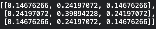
Notice the kernel weights reduce as we drift away from the centre. Hence, when convolved with such a matrix, an image location will lose information from surrounding pixels, leading to smoothing (blur). Besides the gaussian, there are other types of smoothing kernels too. The takeaway here is that a blurry image (B) is a result of some convolution (H) applied to the original image (I).

If we could somehow inverse this operation, we would be able to generate the original image (I). This process is called deconvolution and is easier done in the frequency domain (Fourier transform).
Fourier transform of images
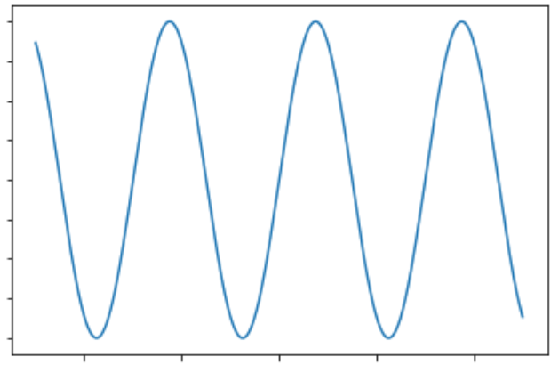
The idea with Fourier transform(FT)is that any function can be approximated as a weighted sum of infinite sinusoids. A 1-D sine wave needs 3 parameters for it’s definition.
- Amplitude (A) determines the range of the wave. It stretches from -A,A
- Frequency (2π/λ) determines the distance between two consecutive peaks
- Phase (φ) determines the horizontal shift in wave
Hence, the Fourier transform shifts a function from spatial domain to frequency domain.
def plot_sine_1D(amp,wavelength,phase):
    x = np.arange(-500, 501, 1)
    y = np.sin((2 * np.pi * x / wavelength)+phase)
    plt.plot(x, y)
    plt.show()
plot_sine_1D(1,300,0)
Any image is a two dimensional discrete function. That is, pixels are a function of their spatial location.
Discrete Fourier transform shifts images to the frequency space where they are represented by 2D sinusoid waves.
def plot_sine_2D(amp,wavelength,phase,angle):
    x = np.arange(-500, 501, 1)
    X, Y = np.meshgrid(x, x)
    wavelength = 100
    sine_2D = np.sin(
        2*np.pi*(X*np.cos(angle) + Y*np.sin(angle)) / wavelength
    )
    plt.set_cmap("gray")
    plt.imshow(sine_2D)
plot_sine_2D(1,200,0,np.pi)
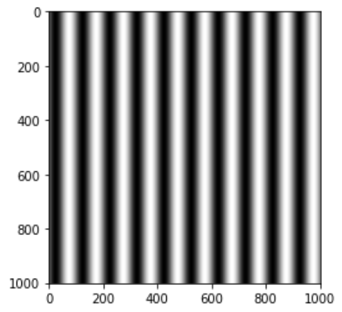
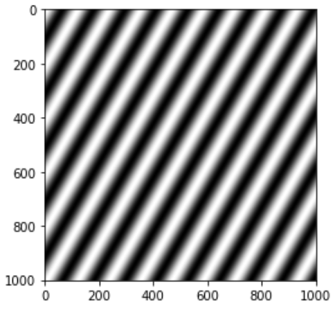
2D sine waves can also rotate with respect to the x,y axes. Below is the same 2D wave rotated by π/6 radians.
plot_sine_2D(1,200,0,np.pi/6)
Let us visualise some Fourier transforms. We use np.fft.fft2 to do that. The second line of the function shifts pixel 0,0 to the centre of the plot and makes visualisation easier. Our array is of size 1001,1001 so the centre is shifted to 500,500. Also, we take the absolute because FT returns a complex number.
def compute_fft(f):
ft = np.fft.fft2(f)
ft = np.fft.fftshift(ft)
return ft
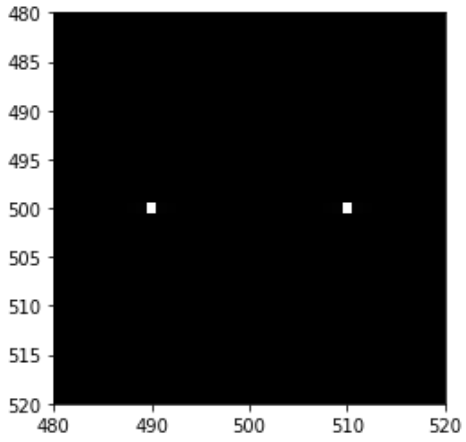
sin = plot_sine_2D(1,200,0,np.pi,False)
ft = compute_fft(sin)
plt.xlim([480,520])
plt.ylim([520,480])
plt.imshow(abs(ft))
sin = plot_sine_2D(1,200,0,np.pi/6,False)
ft = compute_fft(sin)
plt.xlim([480,520])
plt.ylim([520,480])
plt.imshow(abs(ft))
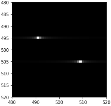
In the first FT, we get two dots at a distance of 10 units from the centre. The distance from the centre represents the frequency. In the second FT plot, we get the same two dots but rotated. The rotation angle represents the rotation of the wave(30 degrees). The pixel values at the the two dots describes the amplitude. Phase information is encoded in the complex part, which we do not plot.
f,ax = plt.subplots(1,2,figsize=(15,20))
ax = ax.flatten()
im = cv2.imread('/kaggle/input/randomimages/pic2.jpeg',-1)
im = cv2.cvtColor(im, cv2.COLOR_BGR2GRAY)
ax[0].imshow(im,cmap='gray')
ax[1].imshow(20*np.log(abs(compute_fft(im))),cmap='gray')
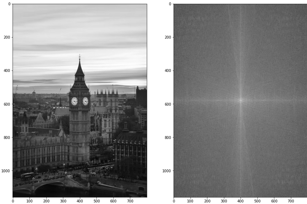
FT of real images are harder to visualize. We do a log operation on the FT to shrink down the values to plot them as an image.
Deconvolution using Fourier transform
We have fussed enough about FTs, but how do they help our case? Well, in the frequency domain, convolution transforms into multiplication. Accordingly, our equation becomes
Or,
Taking the inverse Fourier transform of the RHS should yield the original image. But wait, how to find the correct smoothing kernel (H)? You could try different kernels, depending on the blur. Let’s stick to the Gaussian for now and implement it in code.
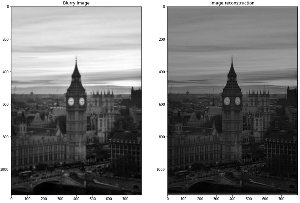
We’ll read in a image and blur it using a 7,7 gaussian kernel with sigma = 5 (standard deviation of the kernel)
# Plotting image and its blurred version
f,ax = plt.subplots(1,2,figsize=(15,20))
ax = ax.flatten()
im = cv2.imread('../input/randomimages/pic1.jpeg',-1)
im = cv2.cvtColor(im, cv2.COLOR_BGR2GRAY)
im_blur = cv2.GaussianBlur(im,(7,7), 5, 5)
ax[0].imshow(im,cmap='gray')
ax[1].imshow(im_blur,cmap='gray')
Next, we’ll define two functions. One to generate a gaussian kernel of given size and another that takes in a blurred image and sharpens it.
def gaussian_filter(kernel_size,img,sigma=1, muu=0):
    x, y = np.meshgrid(np.linspace(-1, 1, kernel_size),
                       np.linspace(-1, 1, kernel_size))
    dst = np.sqrt(x**2+y**2)
    normal = 1/(((2*np.pi)**0.5)*sigma)
    gauss = np.exp(-((dst-muu)**2 / (2.0 * sigma**2))) * normal
    gauss = np.pad(gauss, [(0, img.shape[0] - gauss.shape[0]), (0, img.shape[1] - gauss.shape[1])], 'constant')
    return gauss

def fft_deblur(img,kernel_size,kernel_sigma=5,factor='wiener',const=0.002):
    gauss = gaussian_filter(kernel_size,img,kernel_sigma)
    img_fft = np.fft.fft2(img)
    gauss_fft = np.fft.fft2(gauss)
    weiner_factor = 1 / (1+(const/np.abs(gauss_fft)**2))
    if factor!='wiener':
        weiner_factor = factor
    recon = img_fft/gauss_fft
    recon*=weiner_factor
    recon = np.abs(np.fft.ifft2(recon))
    return recon
Let’s dive deep into the fft_deblur function.
- We generate a gaussian filter of given size and standard deviation .We also pad it with zeros, so that it matches the shape of the image. This is necessary to compute the division in frequency domain
- Compute the FT of blurry image
- Compute the FT of kernel
- Define the Wiener factor. We’ll come to this later. For now, assume it to be 1
- Define the reconstruction as division of (3) and (4)
- Multiply (6) by (5)
- Inverse Fourier transform (7) and compute its absolute value
Let’s analyse the result.
recon = fft_deblur(im_blur,7,5,factor=1)
plt.subplots(figsize=(10,8))
plt.imshow(recon,cmap='gray')
Oops! That did not work. It is so because we did not account for one crucial component — noise. Noise can enter an image from various sources. Accordingly, the blurry image equation modifies to
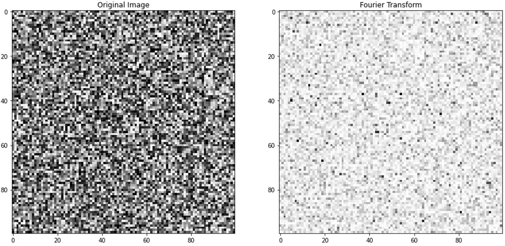
Now while computing the FT of the blurry image(B), we implicitly calculate the FT of the noise component too. The FT of noise has a lot of high-frequency values.
noise = np.random.rand(100,100)
noise_fft = np.fft.fft2(noise)
noise_fft = np.fft.fftshift(noise_fft)
f,ax = plt.subplots(1,2,figsize=(15,20))
ax = ax.flatten()
ax[0].imshow(noise,cmap='gray')
ax[0].set_title('Original Image')
ax[1].imshow(20*np.log(abs(compute_fft(noise_fft))),cmap='gray')
ax[1].set_title('Fourier Transform')
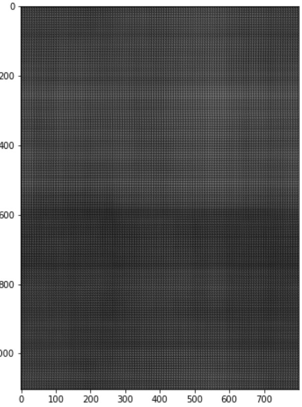
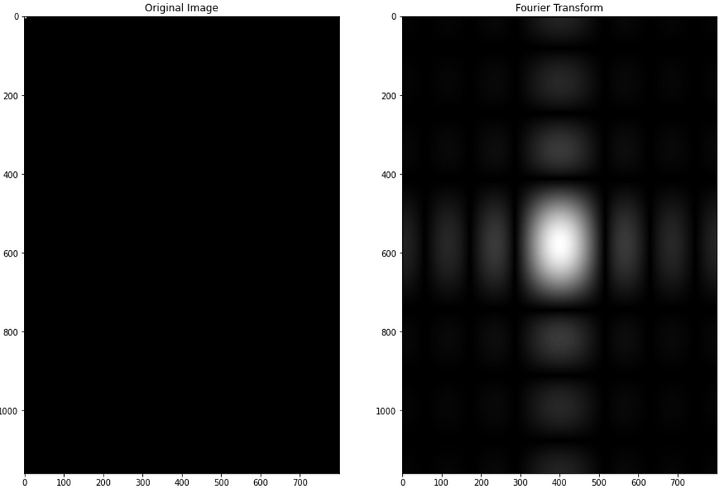
On the other hand, the smoothing kernel has a lot of low-frequency values. As you see in the plot below, if we drift away from the centre, we enter a predominantly black region (0 pixels). Its original image is also mostly black because we have padded it with zeros. There is tiny white region near the top left.
gauss = gaussian_filter(7,im,5)
gauss_fft = np.fft.fft2(gauss)
gauss_fft = np.fft.fftshift(gauss_fft)
f,ax = plt.subplots(1,2,figsize=(15,20))
ax = ax.flatten()
ax[0].imshow(gauss,cmap='gray')
ax[0].set_title('Original Image')
ax[1].imshow(np.abs(gauss_fft),cmap='gray')
ax[1].set_title('Fourier Transform')
Essentially the high-frequency values in FT(B) correspond to noise. When we divide it by FT(H), mostly made up of zeros, we amplify the noise. Hence, we need a regulariser. In comes the wiener factor. You can find more details about the wiener filter here. We can replace 0.002 with any other constant value.
f,ax = plt.subplots(1,2,figsize=(15,20))
recon = fft_deblur(im_blur,7,5,factor='wiener')
ax[0].imshow(im_blur,cmap='gray')
ax[1].imshow(recon)
ax[0].set_title('Blurry Image')
ax[1].set_title('Image reconstruction')
plt.show()
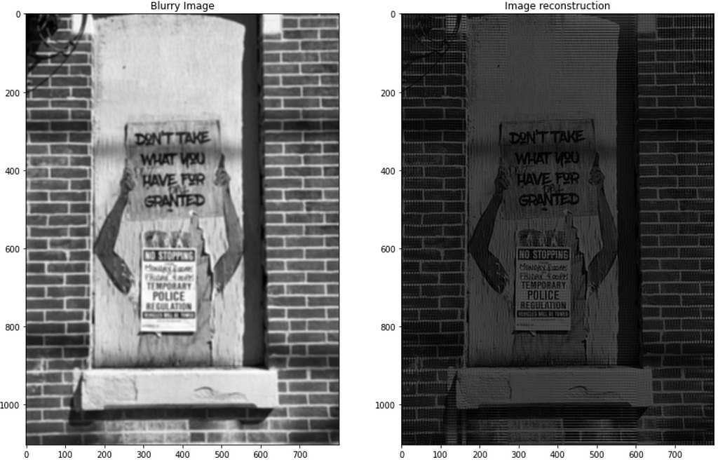
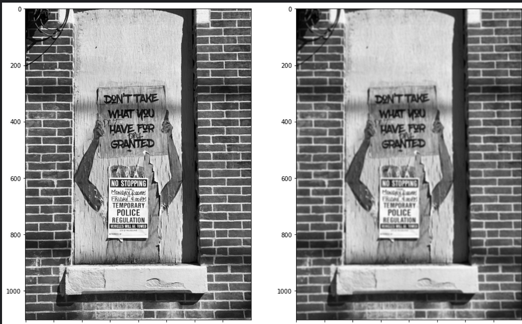
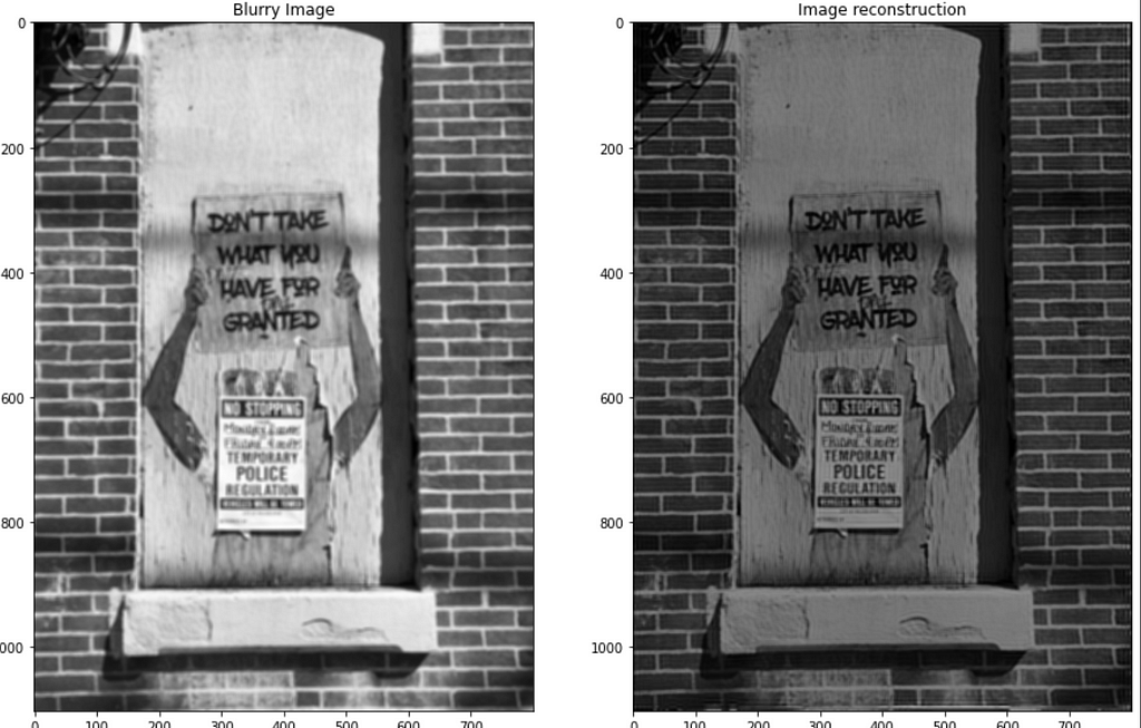
With the wiener factor, we get better results. We can now play with the constant to get clearer reconstructions.
f,ax = plt.subplots(1,2,figsize=(15,20))
recon = fft_deblur(im_blur,7,5,factor='wiener',const=0.5)
ax[0].imshow(im_blur,cmap='gray')
ax[1].imshow(recon)
ax[0].set_title('Blurry Image')
ax[1].set_title('Image reconstruction')
plt.show()
We cannot operate FT on RGB images directly. To unblur RGB images, we can run the deblur function on each colour dimension separately and then concatenate them.
Conclusion
This was a short guide on how to use Fourier transform to unblur images. While an application in itself, deblurring can also be used as an important pre-processing step in a deep learning training pipeline. A thorough understanding of Fourier transform will help anyone working in vision/signal sciences. It is a magnificent algorithm that, according to Veritasium, transformed the world.
References
https://medium.com/media/de5faf9a42a336a991e8f632c61589b1/hrefHow to de-blur images without training neural networks was originally published in Towards Data Science on Medium, where people are continuing the conversation by highlighting and responding to this story.
...