

 800+ IT
News
als RSS Feed abonnieren
800+ IT
News
als RSS Feed abonnieren📚 Machine Learning on Graphs, Part 4
💡 Newskategorie: AI Nachrichten
🔗 Quelle: towardsdatascience.com

Learning discrete node embeddings
In this post, I want to present discrete graph node embeddings as part of my series on machine learning on graphs (part 1, part 2, part 3). In particular, it also discusses my last research paper on discrete node embeddings which was recently accepted for presentation at AAAI 23, the premier conference on artificial intelligence.
In a previous post, I presented the main ideas behind algorithms for learning node embeddings. By default, when we talk about word embeddings in natural language processing or node embeddings in graph learning, we implicitly mean continuous embeddings. Namely, a discrete object like a graph node is represented by a fixed-size continuous vector. For example, a 5-dimensional vector like (0.3, 0.67, -0.9, 0.06, -0.55).
It is well-known that continuous embeddings are a powerful and versatile data representation technique. However, as powerful as continuous embeddings might be, they are not really intuitive for human users.
Consider for example a social network graph where nodes represent users. Each user is described by different attributes such as gender, location, professional experience, personal interests, etc. Continuous node embeddings will utilize this information. For example, London-based software engineers are likely to end up having similar node embeddings because they share many connections in the London area, for example with recruiters or fellow software engineers. However, the continuous embeddings are meaningless to human readers. Most of us cannot compute the cosine similarity or the Euclidean distance between 50 dimensional vectors in our heads.
On the other hand we are good at capturing information by scrolling through larger amounts of text. The idea behind discrete node embeddings is that the embedding vectors can consist of discrete features that are human readable. So, instead by k real values, each node is represented by k discrete features. These features can be node attributes or simply other graph nodes. Then a discrete embedding vector looks like
(software engineer, London, data scientist, Cambridge, chemist)
Each coordinate has a value with a well-defined meaning. In the above we can infer that the user is part of the professional community of UK based professionals with a STEM degree.
We need to address the following questions:
- What makes discrete node embeddings useful in downstream machine learning tasks?
- How to generate discrete embeddings?
- How to train machine learning models with discrete node embeddings?
Useful discrete embeddings
As discussed, discrete node embeddings are easily readable by humans. But in order to use them in interpretable machine learning models, we need to efficiently compare two embedidngs. A first idea would be to randomly collect a set of “close enough” nodes, and/or the attributes describing them, and then use a set comparison operator such as Jaccard similarity. Two node embeddings are similar if the corresponding sets are similar to each other. Such an approach will work but replacing vectors with sets will limit our options for machine learning algorithms that can be used. Also, computing a set intersection is slower than the inner product computation used in continuous embeddings. (Even if the asymptotic complexity in both cases is linear, the set membership operation introduces some computational overhead.) Instead, we set the following requirements.

That is, we require that each coordinate pair is an unbiased estimator for the similarity between nodes. Two embedding vectors are then compared by their Hamming distance, i.e., the number of coordinates on which they differ, the so-called overlap or Hamming kernel. As for the similarity measure between two nodes in the above definition, there are plenty of measures between (attributed) graph nodes. In fact, this is the topic of my previous post where I discussed graph kernels. At a high level, we want nodes that are “surrounded” by nodes with similar characteristics to have similar embeddings. A simple measure for example would be the Jaccard similarity between node neighborhoods approximated by the Hamming kernel.
How to generate discrete embeddings?
The first question is which nodes should be considered “close enough” to sample from. We thus define the k-hop neighborhood of a node to be all graph nodes that can be reached by traversing at most k edges. The 0-hop neighborhood of a node u is thus u itself, the 1-hop neighborhood is the nodes that are connected to u by an edge, the 2-hop neighborhood consists of all neighbors of neighbors, etc.
Having defined the set of nodes from which we are going to sample nodes or node attributes, the next question is how to generate vectors. For example, starting a random walk at each for and traversing k edges would be an option. For an n-dimensional embedding vector, we can start n random walks at each node. But it is easy to see that such embeddings are rather unlikely to have a large overlap. Thus, the formal requirement defined above is not satisfied for a useful similarity measure. We will thus make use of a technique called coordinated sampling [3].
Coordinated sampling is a powerful technique for similarity estimation between sets. Informally, it is based on the idea that if x is sampled from a set A, and if x is a member of another set B, then it is more likely that x is also sampled from B. In this way, the more elements A and B have in common, the more likely are they to end up with the same sample, thus reflecting the similarity between A and B. There are many different coordinated sampling techniques, see for example this presentation. Let us consider a simple technique that makes the above informal description more intuitive.
Coordinated sampling using minwise hashing.
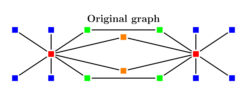
Consider the simple toy graph example in Figure 1. The two red nodes have as common neighbors the two orange nodes. Thus, the Jaccard similarity for the 1-hop neighborhood is 2/16 as all graph nodes are connected to a red node. The Jaccard similarity between the 2-hop neighborhoods is 8/16 as the 8 blue nodes cannot be reached in two hops by one of the red nodes in 2 hops. We want to apply coordinated sampling such that we sample a neighborhood node as a coordinate in the embedding vector for each node.
We will apply minwise independent hashing. We will randomly permute the nodes and take as a sample the first node in the permutation in the neighborhood set. We show how to implement the approach in a very efficient way.
As a first step, we generate a random number between 0 and 1 at each node see Figure 2. The number of random numbers that can be generated in this way is huge (2**32 or 2**64), therefore the order given by the random numbers gives a random permutation on the nodes. For each node, we want to find the node with the smallest random number from its k-hop neighborhood. This will be the sample for the node.
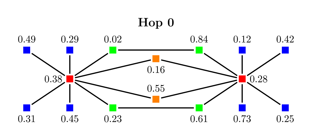
For k=0, we don’t do anything. The 0-hop neighborhood of a node is the node itself.
The 1-hop neighborhood of each node is the set of immediate neighbors of the node, i.e., only nodes that are connected by an edge. In the above, the blue nodes have only one neighbor.
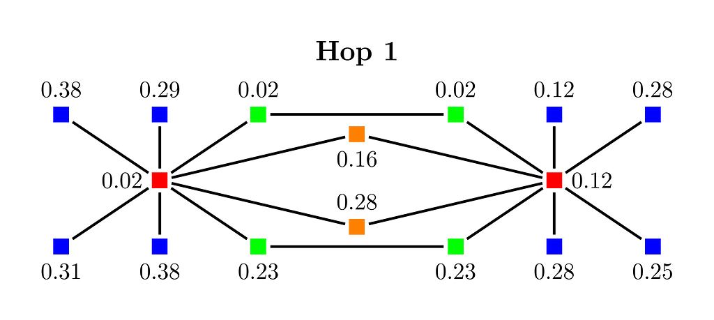
In Figure 3 we see the result after updating each node with the minimum weight of one of its neighbors. For example, the upper right green node has as neighbors a green node with a weight of 0.02 and a red node with a weight of 0.28. Both weights are smaller than its initial weight of 0.84, and we update the red node to have now a weight of 0.02. Similarly, the red node on the right gets a new weight of 0.12 because this is the neighbor with its minimum weight. Note that we don’t update the weight of the node if there is no neighbor node that has a smaller weight than the current node weight.

In Figure 4 we see the result after one more iteration of the approach. The smallest weight 0.02 has reached all nodes within its 2-hop neighborhood. In particular, the two red nodes have now the same sample, namely the green node that originally was assigned the weight 0.02. Observe that if the smallest weight was assigned to one of the blue nodes then the two red nodes would have ended up with different samples. As exactly 50% of the nodes are blue, it is easy to see that each coordinate is an unbiased estimator of the Jaccard similarity between the 2-hop neighborhoods of the two red nodes. And the same reasoning applies to old node pairs. Furthermore, the algorithm is highly efficient. Each iteration takes linear time in the number of graph edges. Thus, for a graph on m edges we need time O(m*k*d) to compute d-dimensional embedding for all nodes by sampling from the k-hop neighborhood of each node.
How to use discrete node embeddings in a machine learning model?
Two typical use cases of node embeddings are link prediction and node classification. Continuous and discrete node embeddings can be used in essentially the same way for link prediction. Predict as new links the node pairs that have the highest similarity scores as given by their embeddings. However, in node classification we a set of labeled nodes and we want to use the embedding vectors to train a model. Thus, we need a classification model that can deal with discrete node embeddings. Clearly, standard choices like logistic regression are not applicable.
Kernel machines. A straightforward choice for node classification is to use a kernel machine with a precomputed kernel matrix [2]. After selecting a subset of the nodes as a training dataset S, we compute the Gram matrix for S, i.e., for each pair of nodes from S we compute the overlap between them. Clearly, this approach can be highly inefficient as it requires memory of O(m²) for m training examples in S. And training a kernel machine with a precomputed kernel might result in time complexity of O(m³).
Explicit feature maps. Let U be the universe from which discrete embeddings can assume values. For example, if node attributes are short text descriptions, then U is the set of all dictionary words. By enumerating all elements in U, d-dimensional embeddings can be described by sparse vectors of dimensionality d*|U|. Even if these vectors are very sparse with only d nonzero entries, using them in a machine learning model will likely result in dense decision vectors, and the approach will become infeasible. Here comes the idea of projecting the embeddings to low dimensional vectors such that I show in the paper that we can project the discrete embeddings to vectors of dimensionality O(d) that approximately preserve the Hamming kernel. You can read more on explicit feature maps in my post on the topic. The main advantage of explicit maps is that we replace the kernel SVM model with a highly efficient linear SVM model using only linear time and space.
Interpretable machine learning.
Supervised learning. Decision trees are the textbook example when introducing interpretable machine learning. Discrete embeddings naturally apply to this setting. For example, we choose as a split the 12-th coordinate of the training vectors and distinguish between two subsets of the values at this coordinate. In the end, we obtain results like: “We predict that the user will download this app because the 12-th coordinate is ‘accountant’, the 8-th is ‘biochemical scientist’, and the 17-th is ‘data analyst”. Overall, this suggests that the user is connected to other users with a technical background and it is thus likely they will use the app in question.
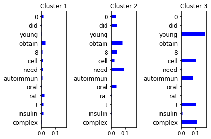
Unsupervised learning. We can cluster the vectors by using an appropriate distance function. Then we can calculate the distribution of features in each cluster. In Figure 5 we show the result after clustering research papers from the PubMed dataset. The nodes in the corresponding graph are the papers and two papers are connected by an edge if one paper cites the other. Each node has as attributes the set of keywords that appear in the abstract of the paper. Thus, embeddings consist of keywords that appear in neighborhood nodes. Note that in the case below we used the explicit feature maps and the distance was the Euclidean distance. Observe that the distribution is shown on a logarithmic scale and shows that the keyword distributions are very different for the three clusters. Thus, we have indeed detected a segmentation of research papers that cite each other and have different topics.
Continuous vs discrete node embeddings.
Let us briefly compare discrete and continuous node embeddings. The advantages of discrete embeddings are:
- Ease and scalability of computation. Discrete embeddings are relatively easy to compute. All we need is a procedure for coordinated sampling from the local neighborhood at each node. In particular, we avoid the need to train a possibly slow word2vec-like model.
- Interpretability. If nodes contain interpretable attributes then the resulting embeddings open the door to interpretable machine learning.
On the other hand, the disadvantages of discrete embeddings are:
- Discrete embeddings are not really versatile. We can use continuous embeddings as input to every conceivable machine learning model while the choices for discrete embeddings are rather limited. Using the explicit map approach described above rectifies the issue. But then the design of interpretable models becomes more challenging, if possible at all.
- Continuous embeddings can capture more information about the underlying structure of the data. Infamous examples for word embeddings like emb(king) ~ emb(queen) + emb(man) — emb(woman) show the capabilities of continuous embeddings to capture more complex relationships. It is unlikely that discrete embeddings can be used to extract such complex relationships from the original graph structure.
More about my AAAI paper and the provided code.
Finally, let me briefly summarize the highlights of my AAAI paper:
- The minwise hashing based approach is rather limited. It only considers if there exists a path between two nodes in the graph, not how many path are there. In the paper, I present local neighborhood sampling algorithms that sample neighborhood nodes according to the number of paths between two nodes.
- A major contribution is that the proposed algorithms have rigorously understood properties. In particular, I provide theorems and an explanation of the similarity measures between nodes preserved by the different sampling approaches.
Some practical advice if you use the implementation:
- A reference Python implementation can be found at https://github.com/konstantinkutzkov/lone_sampler While the implementation is good enough for smaller graphs, for massive graphs it needs to be further optimized. In particular, the embedding generation for different coordinates can be easily parallelized, and thus modern computing platforms can be utilized.
- In order to get an idea of what results to expect, try the minwise hashing approach and the NodeSketch [2] approach which are highly scalable. Use smaller neighborhood depth for minwise hashing, 1 or 2.
- Be careful with bipartite graphs. If you apply the approaches on bipartite graphs, it is recommended to use even hop depth.
- As shown in the experimental evaluation of the paper, the best results are achieved by the more advanced approaches called L1 and L2 sampling. The approaches are rather advanced to be described in a blog post for a general audience. But if you decide to use them, note that the sketch size is in fact a hyperparameter that needs to be tuned. For the experimental evaluation, I used a rather large value for the sketch size as suggested by the theoretical analysis. But the larger the sketch size, the more time and space-consuming the algorithm becomes. It is advised to start with a small value and then increase it to see if there is any practical advantage.
References
[1] Konstantin Kutzkov. LoNeSampler: Local Neighborhood Sampling for Learning Discrete Node Embeddings. AAAI 2023, to appear.
[2] Yang, Dingqi, Paolo Rosso, Bin Li, and Philippe Cudré-Mauroux. NodeSketch: Highly-Efficient Graph Embeddings via Recursive Sketching. KDD 2019
[3] Edith Cohen, Haim Kaplan: What You Can Do with Coordinated Samples. APPROX-RANDOM 2013
Machine Learning on Graphs, Part 4 was originally published in Towards Data Science on Medium, where people are continuing the conversation by highlighting and responding to this story.
...