

 800+ IT
News
als RSS Feed abonnieren
800+ IT
News
als RSS Feed abonnieren📚 Default Hugging Face models are probably all you need for “vanilla” image classification
💡 Newskategorie: AI Nachrichten
🔗 Quelle: towardsdatascience.com
Exploring pre-trained image models on the Hugging Face hub as feature extractors and transfer learners in a land cover classification task
> Code Repo: [link], Notebook: [link]
Intro
In this post, I’ll explore a common practice in representation learning — using pre-trained neural networks in their frozen state as learned feature extractors. Specifically, I’m interested in examining how the performance of simpler models trained on these extracted neural network features compares to fine-tuned neural networks initiated with transfer learning. The intended audience includes data scientists at its core and, more generally, anyone interested in earth observation, computer vision, and machine learning.
To skip forward a little bit… The results below suggest that scikit-learn models trained on extracted neural network features yield nearly comparable performance to full transformers models fine-tuned off the same pre-trained weights (a balanced accuracy dip of -3% to -6%).
Background
Today, the Microsofts of the world release thousands of pre-trained neural networks a year. And, these models are becoming increasingly performant and accessible. With so many model checkpoints open-sourced, the evolution of neural networks as a central focus in AI/ML is not too surprising. Consider that people everywhere have heard about DALL-E-2 and Stable Diffusion — neural networks that can turn text prompts into images/art. Reportedly, Stable Diffusion has already been downloaded by more than 10 million users. What many don’t know is that these technologies exist today in large part due to advances in the subfield of statistics known as representation learning.
“The 2020s are looking like the age of representation learning’s promise being realized in ML. With models trained on a specific domain (either supervised or unsupervised), we can use their late-stage activations in processing input as a representation of their input. Representations can be used in a variety of ways, the most common being used as direct input to a downstream model or used as a target for co-training a shared latent space with multiple types of models (text and vision, GNN and text, etc.).” — Kyle Kranen [1]
Let’s put these claims to the test…
Dataset details
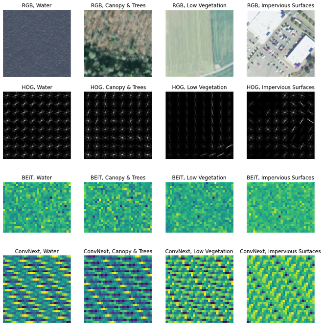
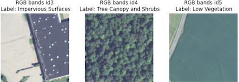
The image dataset used below originates from the 2013/2014 Chesapeake Conservancy land cover project [2]. It is composed of National Agriculture Imagery Program (NAIP) satellite imagery and comes with 4-bands of information at a 1 meter squared resolution (Red, Green, Blue, and Near Infrared). The raw geospatial data originally spans 100,000 square miles across 6 states: Virginia, West Virginia, Maryland, Delaware, Pennsylvania, and New York. It was first subsampled to obtain n=15,809 unique patches of size 128 x 128 pixels and as many land cover labels*. When inspecting example patches (see Figure 1), the 1 meter squared resolution appears fairly fine-grained, since the structures and objects within the images are interpretable at a somewhat high definition.
* Sidenote: The original Chesapeake Conservancy land cover dataset includes label masks — and is intended for segmentation as opposed to classification. To change this, I only saved patches where a single class occurred with at least 85% frequency when sampling the geospatial data. The over-represented class was then recorded as the sole label for that patch, resulting in the simplified 5-way classification problem.
The 5 land cover classes used in the experiments here are defined as…
- Water: Open water areas including ponds, rivers, and lakes
- Tree Canopy and Shrubs: Woody vegetation including trees and shrubs
- Low Vegetation: Plant material less than 2m in height, including lawns
- Barren: Areas of natural earthen material devoid of vegetation
- Impervious Surfaces: Human-constructed surfaces
Upon examination, the dataset appears to have many interesting characteristics including seasonal variation (e.g., foliage), noise (e.g., occasional cloud cover), and distribution shift across the 6 states. The small amount of “natural” noise helps make this somewhat simplified classification task a little more difficult, which is beneficial, since we don’t want the supervised task to be too trivial.
Training, validation, and testing sets were generated using the US states as a splitting mechanism. Patches from Pennsylvania were chosen for the test set (n = 2,586, 16.4% of the data), patches from Delaware were chosen for the validation set (n = 2,088, 13.2% of the data), and the rest were used for the train set (n = 11,135, 70.4% of the data).
Lastly, as a whole, the dataset is somewhat significantly class imbalanced: Barren (49/15,809) and Impervious Surfaces (124/15,809) are highly under-represented and Tree Canopy and Shrubs (9,514/15,809) is highly over-represented. Low Vegetation (3,672/15,809) and Water (2,450/15,809) are more balanced by comparison. Due to this label imbalance, we use balanced accuracy for our experiments below. This metric takes the average of each class’s individual accuracy, thereby weighting each equally regardless of size.
see: torchgeo.datasets
Learned features
In general, learned features can be defined as those that originate from pre-trained models. By extracting learned features from images, you’re effectively entrusting the work of others in the CV community for data representation. For example, one can extract learned features from a neural network pre-trained on a large benchmark dataset (like ImageNet).
Learned features are often excellent representations for downstream tasks, whether it’s unsupervised or supervised — so long as the model’s weights were pre-trained in a robust manner. Luckily, one can trust the Googles/Microsofts/Facebooks for the last bit. For some context, a raw image undergoes several layers of successive transformations when it is fed into a neural network, where each hidden state layer extracts new information from the original image. After feeding an image into the network, one can extract the hidden states or embeddings directly as features. It’s common practice to use the last hidden state embedding as the extracted feature, i.e., the layer that precedes the supervised task head.
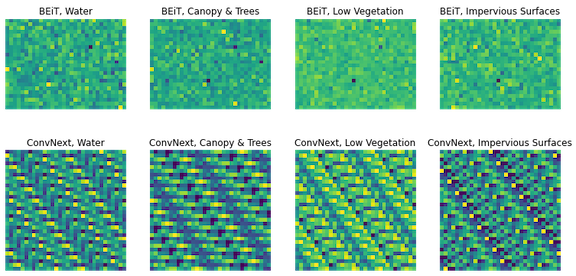
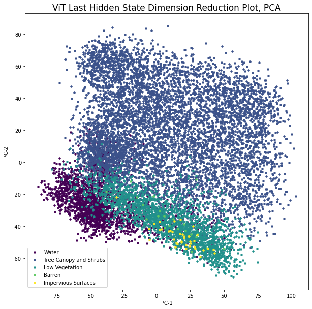
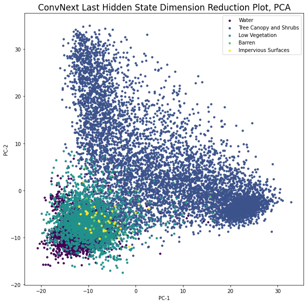
In this project we’ll investigate two pre-trained models: Microsoft’s Bidirectional Encoder Image Transformer (BEiT) [3] and Facebook’s ConvNext model [4]. BEiT-base and ConvNext-base are two of the most popular checkpoints on Hugging Face for image classification and performed well against other options in initial tests. Since extracted hidden states are often of higher dimensionality than 1 x n, a common practice is to take the mean along smaller dimensions to end up with a 1 x n embedding per image. Below, we ended up with 1 x 768 sized embeddings from the base BEiT and 1 x 1024 dimensional embeddings from the base ConvNext. The embeddings were arbitrarily resized to a rectangular shape for visualization, which reveal some different patterns within.
Let’s see how the data presents visually in learned feature space. To do so, we’ll perform PCA on the collection of n image embeddings to transform them into 2-d space. These are then plotted with the class labels as coloring.
see: transformers.BeitModel/ConvNextModel
Modeling
If you go to a Kaggle competition notebook, you’ll find that the most common practice in image classification today is to use the pre-trained weights of the neural networks for transfer learning and fine tuning. In this setting, you first load the weights into a network (transfer learning) and then update it on the new dataset of interest (fine tuning). The latter step is usually run over a few epochs and with a small learning weight, so as to not stray too far from the original weights. However, the transfer learning and fine tuning process often involves more time and more compute compared to using the same models as feature extractors.
The first half of the models below were trained with learned features and scikit-learn models. I employed the following packages to facilitate the full pipeline: from feature extraction (transformers) to model training (sklearn) to hyper-paremeter optimization (optuna). For hyper-paremeter optimization, I searched over various Logistic Regressors and Feed Forward Neural Networks (FFNN) over 10 random trials, which showed that FFNNs with one hidden state of dimensionality 175–200 were usually the best option.
Transfer learned and fine-tuned neural networks were then trained so to compare against these learned feature models, which comprise the second half of the models. I employed the transformers package to fine-tune BEiT and ConvNext base models, the exact same checkpoints as the above. Identical pre-trained weights were used so as to more closely compare “apples to apples” in the experiment.
> See here for Hugging Face’s excellent tutorial on image classification.
see: optuna, sklearn, transformers
Model evaluation
For model assessment, I chose to inspect balanced accuracies, individual class accuracies, and confusion matrices on the held-out test set. The confusion matrices show where the models made mistakes and are helpful for interpretation. Each row represents the examples that are known to exist in the given class (ground truth) while each column represents those that were classified by the model (predictions). The rows sum to the number of ground truths and the columns sum to the number of predictions.
—x — x — x—
Model 1, BEiT embeddings + sklearn FFNN:
Balanced accuracy… 79.6%
+============+=======+========+============+========+=========+
|            | Water | Trees  | Vegetation | Barren | Manmade |
+============+=======+========+============+========+=========+
| Water      |    64 |      0 |          2 |      0 |       0 |
+------------+-------+--------+------------+--------+---------+
| Trees      |     1 |   1987 |          3 |      1 |       0 |
+------------+-------+--------+------------+--------+---------+
| Vegetation |     1 |      3 |        457 |      0 |       0 |
+------------+-------+--------+------------+--------+---------+
| Barren     |     2 |      0 |         14 |      5 |       3 |
+------------+-------+--------+------------+--------+---------+
| Manmade    |     0 |      0 |          6 |      2 |      35 |
+------------+-------+--------+------------+--------+---------+
Class accuracies … Water: 97.0%, Canopy & Trees: 99.7%, Low Vegetation: 99.1%, Barren: 20.8%, Impervious Surfaces: 81.4%.
> The Beit embeddings model performed third best overall.
— x — x — x —
Model 2, ConvNext embeddings + sklearn FFNN:
Balanced accuracy… 78.1%
+============+=======+========+============+========+=========+
|            | Water | Trees  | Vegetation | Barren | Manmade |
+============+=======+========+============+========+=========+
| Water      |    62 |      0 |          4 |      0 |       0 |
+------------+-------+--------+------------+--------+---------+
| Trees      |     2 |   1982 |          6 |      2 |       0 |
+------------+-------+--------+------------+--------+---------+
| Vegetation |     1 |      3 |        457 |      0 |       0 |
+------------+-------+--------+------------+--------+---------+
| Barren     |     1 |      1 |         17 |      4 |       1 |
+------------+-------+--------+------------+--------+---------+
| Manmade    |     0 |      0 |          8 |      0 |      35 |
+------------+-------+--------+------------+--------+---------+
Class accuracies… Water: 93.9%, Canopy & Trees: 99.5%, Low Vegetation: 99.1%, Barren: 16.6%, Impervious Surfaces: 81.4%.
> The ConvNext embeddings model performed worst overall
— x — x — x —
Model 3, fine-tuned BEiT neural network:
Balanced accuracy… 82.9%
+============+=======+========+============+========+=========+
|            | Water | Trees  | Vegetation | Barren | Manmade |
+============+=======+========+============+========+=========+
| Water      |    64 |      0 |          2 |      0 |       0 |
+------------+-------+--------+------------+--------+---------+
| Trees      |     0 |   1986 |          5 |      1 |       0 |
+------------+-------+--------+------------+--------+---------+
| Vegetation |     2 |      3 |        455 |      0 |       1 |
+------------+-------+--------+------------+--------+---------+
| Barren     |     0 |      0 |         13 |      9 |       2 |
+------------+-------+--------+------------+--------+---------+
| Manmade    |     1 |      0 |          6 |      1 |      35 |
+------------+-------+--------+------------+--------+---------+
Class accuracies… Water: 97.0%, Canopy & Trees: 99.7%, Low Vegetation: 98.7%, Barren: 37.5%, Impervious Surfaces: 81.4%.
> The fine-tuned BEiT model performed second best overall
— x — x — x —
Model 4, fine-tuned ConvNext neural network:
- Balanced accuracy… 84.4%
+============+=======+========+============+========+=========+
|            | Water | Trees  | Vegetation | Barren | Manmade |
+============+=======+========+============+========+=========+
| Water      |    65 |      0 |          1 |      0 |       0 |
+------------+-------+--------+------------+--------+---------+
| Trees      |     0 |   1978 |         12 |      2 |       0 |
+------------+-------+--------+------------+--------+---------+
| Vegetation |     1 |      2 |        457 |      0 |       1 |
+------------+-------+--------+------------+--------+---------+
| Barren     |     0 |      0 |         13 |     11 |       0 |
+------------+-------+--------+------------+--------+---------+
| Manmade    |     0 |      0 |          7 |      2 |      34 |
+------------+-------+--------+------------+--------+---------+
Class accuracies… Water: 98.5%, Canopy & Trees: 99.3%, Low Vegetation: 99.1%, Barren: 45.8%, Impervious Surfaces: 79.1%.
> The fine-tuned ConvNext model performed best overall 🚀🤖
— x — x — x —
Improvements to Modeling Process / Limitations
The modeling pipeline could have been improved in a number of areas, including those discussed next. The models suffer most in classification of the Barren examples, so I would start by adding more of this type of class if I could make a single change. As is, the models are really more like 4-way classifiers since the Barren class performance is so poor. Another improvement could have been using cross validation in the hyper-parameter optimization; yet, cross-validation would have taken a longer time to run and felt like overkill for this experiment.
Generalization limitations of the outputted models include worsened classification performance on imagery of other class types, at other resolutions, and with other conditions (new objects, new structures, new classes, etc.). I’ve gone ahead and pushed the fine-tuned ConvNext and BEiT to Hugging Face for hosted inference, where one can test the generalizability of the models by loading images and/or running the defaults configured within each.
Project Learnings
- Knowledge of the Python package universe is critical. See the grayed-out chunks below for the various libraries used herein.
- Visualizing variation across image features provides a deeper understanding of signals in datasets.
- Pre-trained embeddings paired with simpler models can perform nearly as well as fine-tuned neural nets.
- Hugging Face is not only great for Natural Language Processing, it’s also amazing for Computer Vision!
Conclusion
What do these results and learnings suggest about the state of neural networks in CV today? Let’s rewind. In 2017, the former director of Tesla’s self-driving unit Andrej Karpath wrote a now-famous blog post on the shift from the old school engineering to the new school of deep learning, which he dubbed “software 2.0” [5]. From this viewpoint, neural networks aren’t “another tool in your machine learning toolbox”. Rather, they represent a shift in the way we can develop software. I believe that software 2.0 is as relevant today as it was five years ago. Just look at the number of neural networks available open-source in NLP, CV, and beyond from the top research labs in AI/ML. For practitioners, this is exciting stuff…
Citations
[1] K. Kranen (2022), The 2020s are looking like the age of representation learning’s promise being realized in ML, LinkedIn.
[2] Chesapeake Bay Program Office (2022). One-meter Resolution Land Cover Dataset for the Chesapeake Bay Watershed, 2017/18. Developed by the University of Vermont Spatial Analysis Lab, Chesapeake Conservancy, and U.S. Geological Survey. [Nov 15, 2022], [URL],
- Dataset License: The dataset used herein is publicly available to all without restriction. See here and here for more information.
[3] Bao, H., Dong, L., & Wei, F. (2021). BEiT: BERT Pre-Training of Image Transformers. CoRR, abs/2106.08254. https://arxiv.org/abs/2106.08254
[4] Liu, Z., Mao, H., Wu, C.-Y., Feichtenhofer, C., Darrell, T., & Xie, S. (2022). A ConvNet for the 2020s. CoRR, abs/2201.03545. https://arxiv.org/abs/2201.03545
[5] A. Karpath (2017), Software 2.0, Medium.
[6] Nanni, L., Ghidoni, S., & Brahnam, S. (2017). Handcrafted vs. non-handcrafted features for computer vision classification. Pattern Recognition, 71, 158–172. doi:10.1016/j.patcog.2017.05.025
— x — x — x —
Appendix
Non-learned Features
Non-learned features in CV can be thought of as those that are handcrafted from images [6]. The best non-learned features for a given problem often rely on knowledge of where differentiating signals lie in the dataset. Let’s plot some random patches in RGB space first, before we extract non-learned features.
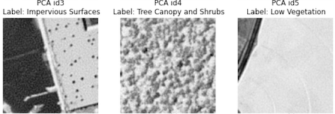
We’ll investigate Principal Component Analysis (PCA) as the first non-learned feature. PCA is a technique for dimension reduction — here, we use it to move from 128 x 128 x 4 images to 1 x n vectors. The size n of the PCA transformed dataset is user-specified and can be any number less than the original dimensionality of the data. Under the hood, the algorithm uses eigenvectors (directions of spread in the data) and eigenvalues (relative importance of directions) to find the set of bases that retain the most variance from the original images. Once calculated, PCA can be employed to transform new images into a lower dimensional space and/or to visualize images in two or three dimensions (see Figures 3 and 4).
In the examples below, PCA with n=3000 dimensions kept resulted in 95% savings in dimensionality while preserving nearly all of the signal from the raw images. To visualize the PCA, I inversed the operations and plotted examples as 128 x 128 pixel images.
Let’s look at another old-school feature: Histogram of Gradients (HOGs). To calculate HOG, gradients (intensity of change) and orientations are first calculated across an image. The image is then partitioned into a number of cells where orientations are stratified into histogram bins. Then, at each pixel in a cell, we look up its orientation, find the corresponding bin in the histogram, and add the given value to it. This process is then repeated across the cells of the image. And, Voila.
Check out the cool things HOG is doing here:
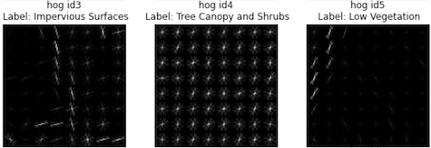
While these handcrafted features are interesting to inspect as a first pass visualization of the dataset, it turns out that they aren’t so great for our supervised modeling purposes. Here, initial tests suggested that models constructed from HOG and PCA features incurred a significant drop off in balanced accuracy relative to the models trained from learned features explored below (35% decrease for PCA, 50% decrease for HOG).
see: skimage.feature.hog, sklearn.decomposition.PCA
Default Hugging Face models are probably all you need for “vanilla” image classification was originally published in Towards Data Science on Medium, where people are continuing the conversation by highlighting and responding to this story.
...