

 800+ IT
News
als RSS Feed abonnieren
800+ IT
News
als RSS Feed abonnieren📚 Understanding Diffusion Probabilistic Models (DPMs)
💡 Newskategorie: AI Nachrichten
🔗 Quelle: towardsdatascience.com
Building, step by step, the reasoning that leads to DPMs.

This post was co-written with Baptiste Rocca.
Views and opinions expressed are solely those of the authors and do not express the views or opinions of their employers. Unless otherwise noted, all images are by the authors.
Introduction
Modelling complex probability distributions is a central problem in machine learning. If this problem can appear under different shapes, one of the most common setting is the following: given a complex probability distribution only described by some available samples, how can one generates a new sample?
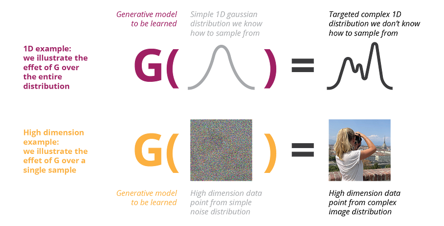
All generative models rely on the same underlying idea that consists in transforming a simple distribution into the complex distribution we are interested in. In other words, assuming that a random variable X follows a simple distribution (for example a gaussian), we are looking for a function G such that G(X) follows our target distribution. Of course, the function G is very complex and can’t be given explicitly. A possible approach is to model G with a neural network that will be learned from available data. We then talk about deep learning generative models like VAEs, GANs or DPMs that all rely on different mechanisms to define and train this generative network that models G.
Back in 2013, Kingma and Welling introduced Variational AutoEncoders (VAEs). In a nutshell, the idea of VAEs is to train an autoencoder with a regularised latent space. The regularised encoder is then forced to encode data towards a distribution close to a gaussian whereas the decoder reconstructs data from the latent space. Doing so, we end up with a decoder that can serve as our function G, taking data from a Gaussian distribution and generating a new data from the original distribution. More details can be found in our previous article about VAEs.
A year later, in 2014, Ian Goodfellow introduced Generative Adversarial Networks (GANs). In short, the idea is to assume that if a generative network G produces samples from the target distribution, then these samples should be indistinguishable from the true available samples. So the concept of adversarial training GANs rely on can be derived. A generative network G is trained to take a random input (from a gaussian, for example) and to output a data from the target distribution. A discriminative network D is trained to differentiate true data from generated data. Both models are trained at the same time and become better while competing (G trying to fool D, D trying not to be fooled by G). During this training process G has to produce always more convincing data to fool D, in other words data that follow the target distribution, as expected. More details can be found in our previous article about GANs.
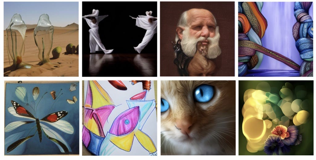
If deep learning generative models have received a lot of attention for many years already, they have been even more exposed in the recent years (or even months) with the raise of some images or videos generation models capable of outstanding results. One after the other, big tech actors have first released image generation models (DALL-E 2 from Open AI, Imagen from Google, Make-A-Scene from Meta) before attacking the videos generation problem (Imagen Video from Google, Make-A-Video from Meta). Despite their differences, these great models announcing a bright future for this field all rely on the same underlying concept: Diffusion Probabilistic Models (DPMs).
Diffusion Probabilistic Models have first emerged in 2015 with a paper of Sohl-Dickstein and have gained more and more traction due to the great results that have been achieved using them. Basically the idea of DPMs is to learn the reverse process of a well defined stochastic process that progressively destroy information, taking data from our complex target distribution and bringing them to a simple gaussian distribution. Such reverse process is then expected to take the path in the opposite direction, taking gaussian noise as an input and generating data from the distribution of interest.
Without further ado, let’s (re)discover DPMs together!
Outline
In this article we will focus on the main ideas required to understand in depth what DPMs are made of. In the first section we will review some notions related to stochastic processes and introduce what is a diffusion process. Then, is the second section we will give the main intuitions to understand diffusion probabilistic models. In particular we will see how diffusion process can be used to destroy information progressively and how we can learn to reverse this process to progressively generate information from noise. In the third section we will formalise our intuitions and give a mathematical description of diffusion models. Finally in the last section we will build on top of this theoretical framework and see how diffusion models are trained in practice. In particular, we will close the loop and see how practical implementations of training and sampling express pretty well the first intuitions we gave. Notice that despite we will discuss many basic notions they rely on, we won’t enter into the details of the specific models mentioned earlier (Make-A-Scene, Imagen, DALL-E 2, etc.) that will be the subject of a future post.
Note: Some sections of this post are more mathematically intensive than others. If all the sections are not completely independent from each others, we tried as much as possible to make it possible for the reader to skip some parts. The section that introduce diffusion processes and the section that give a mathematical definition of diffusion models can then be skipped as the other two sections are containing most of the intuitions and practical considerations related to diffusion models.
What is a diffusion process?
As suggested by their name, diffusion probabilistic models are related in some way to diffusion processes. So let’s start by the very beginning and see what a diffusion process is and what are its properties. Of course, as it is not the core subject of this post, we will have to make some simplifications to keep this short enough while still giving the basic ideas.
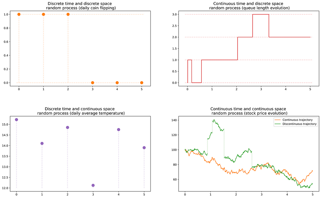
A diffusion process is a continuous time Markov stochastic process with continuous sample paths. Let’s break down this pretty awkward definition to get a better idea of what we are talking about. A stochastic process is a collection of random variables that is most often indexed either by positive integer

we then talk about discrete time stochastic process, or by positive real

we then talk about continuous time stochastic process. Similarly to a realisation of a simple random variable that is called a sample, we call a realisation of a stochastic process a sample path, or a trajectory. For a continuous time stochastic process, we say that it has continuous sample paths if all the possible trajectories that can be randomly observed are continuous.
Finally, a Markov process is a stochastic process with no memory. It means that the future behaviour of the process according to the present and the past only depends on the present. Past information can be discarded as it doesn’t give any additional information. In other words, the future state of the process doesn’t depends on how we get to the present state but only on this present state. Mathematically, it can be written

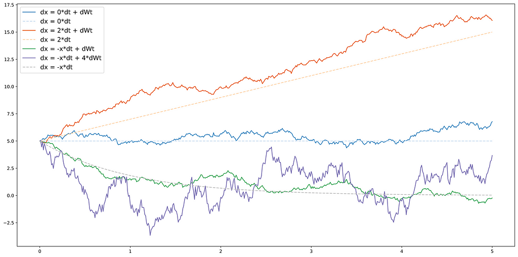
Any diffusion process can be described by a stochastic differential equation (SDE) that is written under the following form

where a is called the drift coefficient, σ is called the diffusion coefficient and W is the Wiener process. The Wiener process is better known as Brownian motion. Roughly speaking, the right part of the sum, related to the Wiener process, is what makes this differential equation “stochastic”. Without this second term, we would deal with a simple differential equation. The Wiener process brings some (continuous) randomness with independent gaussian increments such that

If we discretise a little bit the differential equation to make things easier to grasp, we got

that can also be written

We can then see that the value of X_{t+dt} is the value of X_t to which we add a deterministic drift term and a stochastic diffusion term defined by a normal random variable with variance proportional to the diffusion coefficient squared. So, the diffusion coefficient indicates the strength of the randomness to be applied.
Finally, let’s conclude by an interesting property of diffusion processes that will be useful later in this article. If X_t is a diffusion process such that

then the reversed-time process X̄_t = X_{T-t} is also a diffusion process with the same functional form, described by the following stochastic differential equation

where p(X_t) defines the marginal probability of X_t and

is called the score function.
Intuition of diffusion models
With some well chosen coefficients, a diffusion process has the effect to progressively destroy any relevant information. Indeed, a diffusion with a “shrinking” drift coefficient (|a|<1) and a non-null diffusion coefficient will progressively turn data from any complex distribution into data from a simple isotropic gaussian noise (gaussian whose covariance matrix is diagonale, meaning that all dimensions are independent gaussians). Let’s first illustrate this with a simple 1D example.
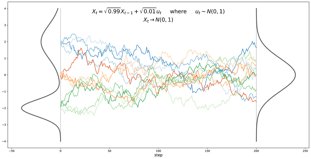
In this 1D example, we have defined the “discretised diffusion process” as being

and we say that for any X_0 this process will ultimately tends towards a gaussian distribution. Let’s give an informal demonstration of this fact that will also justify these square roots in our coefficients. After a given number of steps T we can write

where all the gaussians are independents, meaning that the second term can be expressed as a single gaussian whose variance is the sum of all the variances. For a number of steps T large enough, we have

We see that the first term becomes negligible and the sum of the variances converges towards 1, meaning that for any starting point we tend towards a standard gaussian distribution in our 1D example.
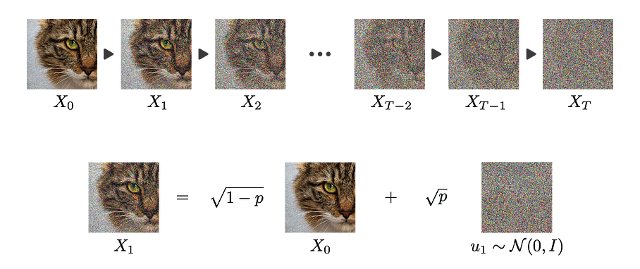
Of course, the same idea can be applied in much higher dimension. For example, the distribution of images of size 100*100 is a very complex high dimensional distribution that can be progressively turned into a very simple distribution of same dimensionality: 100*100 isotropic noise. In such case, the diffusion process will act in a similar way to what we described in our 1D example but it will do so for each RGB channel of each pixel.
So far, we know that we can use a diffusion to go from a complex distribution to a simple isotropic gaussian noise. From what we discussed at the beginning of this article, one could outline that we are much more interested in the reverse process: going from the simple distribution to the complex one. On top of that, going from complex to simple distribution is not that hard as we could simply randomly project any point of the complex distribution into the simple distribution as we know how to sample from this last one.
So what is really the point of using a diffusion here? The simple answer is that it gives us a progressive and structured way to go from our complex distribution to an isotropic gaussian noise that will ease the learning of the reverse process. Let’s get an intuition of that last point.
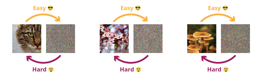
As we mentioned, it is pretty easy to randomly project any given image to an isotropic gaussian noise. On the contrary, reversing the process is very difficult: looking at some given noise we can’t say much from the prior image as there is no structure to rely on.
Now let’s assume that each of these images are not directly, but progressively projected to an isotropic gaussian noise through a diffusion process. Looking at the final step, which is basically noise as we got before, we still can’t say much. However looking at intermediate steps, we clearly have some clues to guide us to reverse the process.
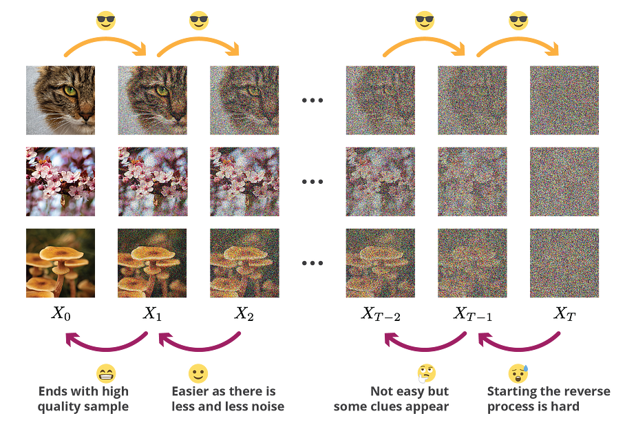
And this the important point here: intermediate steps are the strength diffusion model rely on. At this point one could have indeed observed that despite the fact it is done progressively, diffusion process ultimately take any data point from the initial complex distribution and turns it into a random point from the simple distribution. So, in the end, as we can go from complex to simple distribution in one shot, why bothering with intermediate steps? Instead of learning a multistep reverse process, why not learning a single big reverse process that would be the unrolled version of the multistep process? Can’t we even consider that it would be exactly the same?
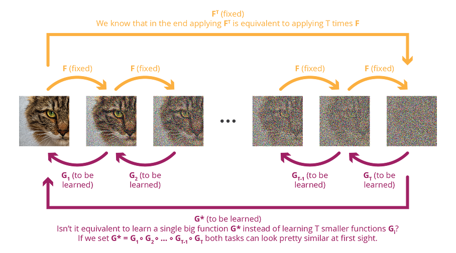
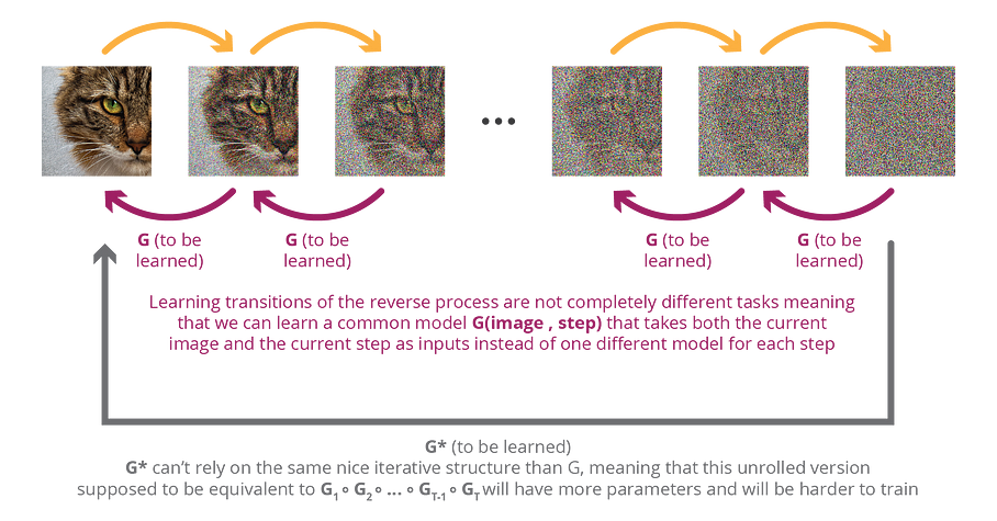
If one could be tempted to hold this reasoning, truth is that breaking down the process into intermediate steps brings two things. First, all the reverse steps are not completely different from each others, meaning that in practice we don’t have to learn a fully different model for each reverse step but instead a common model that simply takes the step as a parameter to adjust its behaviour. It drastically reduces the size of the model to be learned. Second, on top of having much more parameters to be learned, a one shot unrolled version is much harder to train as it needs to go from pure noise to final high quality data, making the task and gradient descent learning much more complicated. At the opposite, a progressive model do not need to handle the whole complexity at once and can first introduce coarse information at the early stages before adding progressively finer and finer information. Intermediate steps can in some sense also be seen as a way to guide the training process to make it easier.
We can then summarise the main idea of diffusion models as follows. We define a diffusion process that destroys information progressively and learn its reverse process expected to restore information. This reverse process is also progressive and we can rely on that fact to make its learning more efficient. In practice, both modelling and training can indeed take advantage from the iterative nature of the process to be learned, compared to a one-shot model that can’t rely on these valuable intermediate steps.
Taking a step back, we can observe that the overall idea is not that far to what is done with VAEs: an encoder transform initial complex distribution into a simple distribution in a structured way in order to be able to learn a decoder that takes the opposite direction. The main differences between DPMs and VAEs are the following. First, the encoder is a multiple step process and not a single step encoder. Second, the encoder is fully fixed and requires no learning due to the fact that the decoder to be learned (the reverse process) will directly rely on the structure brought by the diffusion process instead of relying on a structure learned during the training. Third, the latent space has the exact same dimension as the input, contrarily to the latent space of a VAE whose dimensionality is orders of magnitude lower than the encoded input. Finally, the learned decoder is the reverse process of the diffusion process and, so, is a multiple step process instead of a single pass function.
The obvious downside of DPMs is that sampling requires multiple steps, meaning that the generative process will be longer than it is for GANs or VAEs, as these kind of models require a single pass. This fundamental difference raises many questions. Assuming an equivalent number of parameters, is it completely fair to compare DPMs outputs with GANs and VAEs outputs when the first one make several passes (and, so, takes more time) ? How much sense does it make to try to distillate DMPs if their strength come from the progressive nature of their generative process? We won’t answer these questions here, but they are, for sure, interesting ones to think about.
Mathematics of diffusion models
Now that we have built the intuition, let’s give a more formal mathematical formulation of DPMs. Despite both continuous and discrete time formulation of diffusion models exist, we will focus in this post on the later. It means we will assume that the forward diffusion process and the backward reverse process have been discretised into a finite number T of steps. Notice that for both the forward and the reverse process it is then more accurate to talk about Markov chain with gaussian transition probability kernel instead of diffusion process, but the idea is the same.
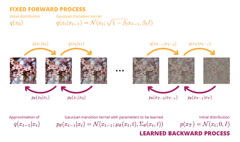
Let’s denote x_0 a data from a distribution we want to sample from and q(x_0) the distribution itself. We define the forward process with gaussian transition probability (the diffusion kernel) as follows

where β_t indicates at each step the trade-off between information to be kept from the previous step and new noise to be added. We can also write

where we can clearly recognise a discretised diffusion process. We can easily show with a simple recurrence argument that any step from the chain can be directly generated from x_0 according to

where

From the Markov property, we can write the probability of a given forward trajectory as

A we described in the previous subsection, our goal is to learn the reverse process of this forward diffusion process, or, more exactly, the reverse chain of this forward Markov chain. We mention earlier that under some assumptions on the drift and the diffusion coefficient (that are met here) the reverse of a diffusion process is also a diffusion process of the same functional form (with the same diffusion coefficient, but we will come back to that later). With sufficiently small time steps (large T, implying small β_t) we can make the approximation that same property holds for the reverse chain we are looking for, that should then also be a Markov chain with gaussian transition probability. The reverse process

can then be approximated by

where µ_θ and Σ_θ are two functions parametrised by θ to be learned. Using the Markov property, the probability of a given backward trajectory can be approximated by

where p(x_T) is an isotropic gaussian distribution that does not depend on θ

Now that we have defined our forward process and modelled its reverse process comes the big questions. How do we learn µ_θ and Σ_θ parameters? What is the loss to be optimised? What we mainly expect from the reverse process is that p_θ(x_0) be close to q(x_0). In other words, the distribution of generated data after the final sampling step of the reverse process should be the same as the targeted distribution. So the learning of the reverse process consists in finding µ_θ and Σ_θ that minimise the KL divergence between q(x_0) and p_θ(x_0), or equivalently that minimise the negative log likelihood of p_θ(x_0) under q(x_0). Mathematically, we want to find µ_θ and Σ_θ that minimise

At this stage it is still not clear where intermediate steps come into play but it will soon be. Let’s first rework the expression in parenthesis a little bit.

Then, the log function being concave, we have from the Jensen inequality

and, so, we can define a higher bound to L

Instead of minimising L we can then minimise the upper bound of L that is easier to deal with. At this point of the derivation it already gets clearer how we can, at least from a theoretical point of view, learn the parameters of our reverse process by iteratively sampling from the forward process and adjusting the parameters to minimise the negative log ratio in the upper bound. However let’s make a last effort and push the derivation a bit further to obtain a more convenient form of this upper bound.

Using the Bayes theorem we have

and so

The first term doesn’t depend on µ_θ and Σ_θ and so doesn’t need to be considered in the optimisation process. The last term is pretty self-explanatory and is not that hard to optimise. Finally, the remaining terms are KL divergence between gaussian distributions. Indeed, we already saw that

and we can show that

where

The KL divergence between 2 gaussian distributions having a closed form, we will see in the next section that this upper bound defines a very tractable loss function to be minimised for the training process.
Diffusion models in practice
So far we have defined a forward process q acting as our (discretised) diffusion process that progressively destroy information

as well as a backward process p_θ modelling the reverse process to be learned and supposed to progressively restore the information

We have then seen that training our reverse process consists in finding µ_θ and Σ_θ that minimise the upper bound

At this point it is worth noting that the different terms in the upper bound expression are independent from each others if we omit that parameters of the reverse model to be learned are shared between steps. So, assuming enough capacity from our model, minimising the entire upper bound is similar to minimising each of its terms.
Let’s now make some assumptions and see how training can be done in practice. First, in order to make things easier, we can decide to set the variance of our reverse process to an untrained time dependent constant such that

The first option matches the variance of q(x_{t-1} | x_t) under the assumption that time steps are small enough (large T, implying small β_t) and, so, that the reverse process has the property to have the same “diffusion coefficient” than the forward process. The second option matches the variance of q(x_{t-1} | x_t, x_0). In practice, studies seem to show that both options give similar results. We will assume the second option for now.
It only let us with a single model to be learned for the mean of the reverse process. Reminding that

it can be shown, using the closed form of the KL divergence of two gaussians, that

We can then see that each KL divergence term of the upper bound corresponds to a given time step and its optimisation simply consist in minimising the L2 distance between the model and the mean of the reverse process conditioned on x_0, both evaluated at the considered time step.
If this formulation is already pretty convenient, it is often preferred to reparametrise the model in terms of noise. First, we notice that

It implies that

and, so, we can reparametrise the model by defining

so that

With this new parametrisation, we no longer learn a model that represent the mean of the reverse process but a model that represent the noise that has been added into x_0 to get x_t. The minimisation of each KL divergence terms of the upper bound now consists in minimizing the L2 distance between the model and the noise.
So far we have omitted the last term in the upper bound we want to minimize

Despite it requires some attention to be handled in a proper way, this term can also be nicely expressed in terms of either µ_θ(x_1, 1) or ε_θ(x_1, 1) depending on the chosen parametrisation. Finally, the overall expression is then well differentiable with respect to the model parameters θ and the training can be done by minimising this upper bound.
However, if the exact upper bound can be used for the training, the following simpler variant has been suggested and is often used in practice

This variant defines a much simpler loss function to be implemented and has been proven to be beneficial to the sample quality.
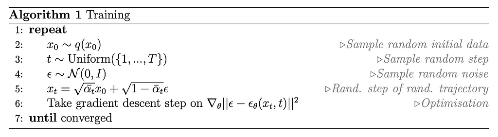
As a major difference with the initial upper bound, one can observe that the expectation is no longer over an entire random forward trajectory but over a random triplet (initial data, step, noise) that defines a single step of a random forward trajectory. Such a change can be explained by the independence of the terms in the upper bound (ignoring the fact that parameters to be optimised are shared). As we already mentioned earlier, this independence implies that minimising the entire upper bound is equivalent to minimising each of its terms. During the iterative training process, it is then theoretically similar and practically much easier to sample a single step and optimise the corresponding term than sampling a complete forward trajectories and optimising for all the terms. That is one of the reasons that makes this variant so appealing.
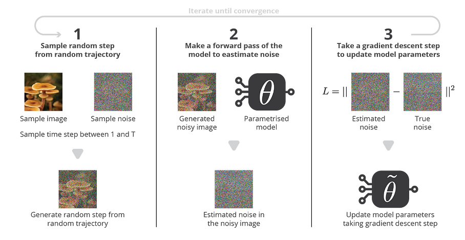
At the end of the day, we are left with this very neat loss function to be optimised. The neural network modelling the noise can take almost any shape depending on the nature of the data. In the case of images, many papers use convolution and attention blocks organised in a U-Net shape, but other architectures could also fit. Then the training simply consists in iteratively sampling some triplets (initial data, step, noise) and applying a gradient descent step with respect to the loss function.
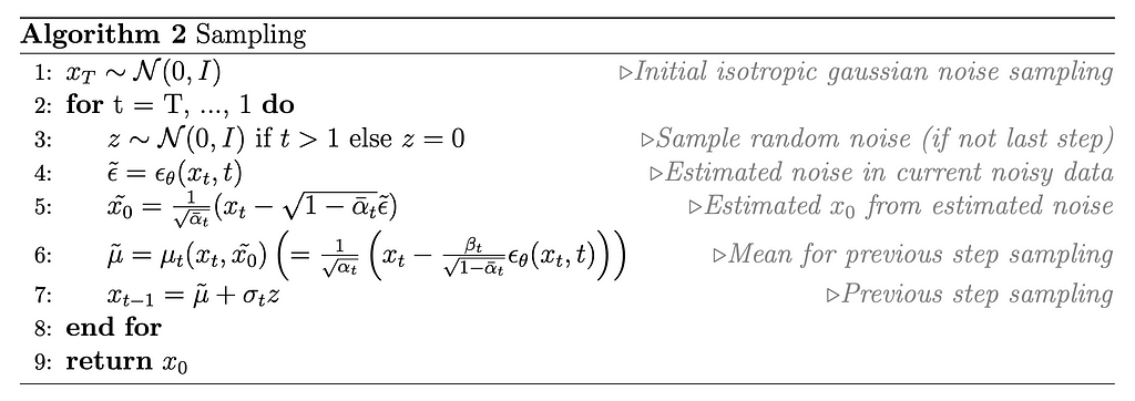
At sampling time, we will start by sampling some noise from the isotropic gaussian distribution and, then, we will use our learned reverse process to generate a data from the target distribution. At each step of the generation process, the parametrisation in terms of noise implies that the model takes both the noisy data and the current step and estimates the noise component. An approximation of x_0 can then be computed and used to define the mean of the reverse process conditioned on this approached x_0.
At first sight, one could have spotted some puzzling behaviour in our sampling process: at the very first step (and all the following steps, in fact) we estimate the noise in the noisy data, making possible to compute an estimate of x_0. So why bothering with all the next steps? Why not only keeping the first estimated x_0 as our final data to be returned? The answer is that the model is simply not assumed to be powerful enough to remove all the noise in one shot. So, the first estimate of x_0 is not expected to be perfect, but it indicates a coarse direction to follow for the next sampling step, as we will sample from the reverse process conditioned on this estimate.
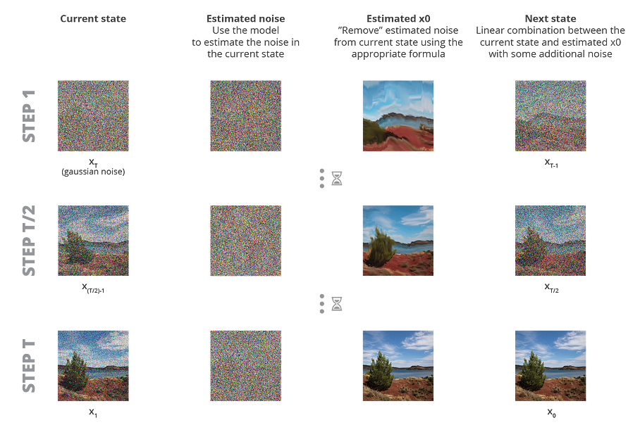
The formula of the mean of the reverse process conditioned on x_0 (µ_t(x_t, x_0)) is a linear combination between x_t and x_0 (see equation above) that clearly indicates the fact that our next sampling step x_{t-1} will be in some way a mix between the current step and the estimated x_0. One could say very roughly that we will sample the next step “somewhere in between the current step and x_0”. With this in mind, we can imagine our generative model as follows: first we sample a final step x_T from random noise, then, step by step, we estimate x_0 from the current state and generate the previous step based on the current state and with this estimate as some kind of “target”. A we mentioned, at the first steps the x_0 estimate won’t be good because the model is not expected to have the predictive power to do so, but iteration after iteration these estimates will guide the reverse generative process and will become better and better, until we get a high quality final sample.
Finally, we can bridge the gap between the first intuitions we built and the more formal description of DPMs we just gave. We can see “in the maths” the advantages of a progressive generation process like DPMs over a single pass generation process. The trained model do not need to handle the all generation in one pass. Instead, the model can first introduce coarse information at the early stages before adding progressively more and more details while it keeps denoising. On top of that, when modelling this reverse denoising process we exploit the fact that denoising images with different levels of noise are not completely different tasks and rely on similar mechanisms that can be mutualised and learned through a single neural network.
Takeaways
The main takeways of this article are:
- generative processes all aim at the same goal that consists in defining a function that takes data from a simple distribution and convert it into data from a complex distribution
- learning a function (represented by a neural network) that takes some gaussian noise and output data from a targeted complex distribution can be a pretty difficult task
- diffusion processes, or their discretised version, Markov chains with gaussian kernels, can be used to progressively destroy information, meaning that they can be used to take data from a complex distribution (e.g. meaningful images) and progressively turn them into data from a very simple distribution (e.g. gaussian noise) by adding noise
- the idea of diffusion probabilistic models is to learn the reverse process of a diffusion, expected to go progressively from some gaussian noise to a complex distribution by removing noise
- the iterative nature of the task makes it simpler as the trained model does not need to handle the whole generation in one pass and can first introduce coarse information before adding progressively more and more details while it keeps denoising
- the model to be learned relies on the fact that denoising images with different levels of noise are similar tasks relying on common mechanisms that can be shared through the training of a single neural network
In this article we have described the main concepts to understand the basics of diffusion probabilistic models. Of course there remains a lot of knowledge to be explored, going from possible improvements over the basic setup we described in this post, to the idea of Denoising Diffusion Implicit Model (DDIM), passing by the notions of conditioning and guidance (classifier based and classifier free) that are at the heart of the amazing generative models that we can see everywhere on the internet these days.
This post is already pretty long and dense. So it would have been too much information to enter into details of more advanced mechanisms related to DPMs here. However, we highly encourage the interested reader to read the papers linked above to deepen its knowledge and its understanding of the field with great content. And, maybe, we will write another article to tackle these notions we left on the side for now… going step by step, like our DPMs.
Thanks for reading!
Other articles written with Baptiste Rocca:
Understanding Diffusion Probabilistic Models (DPMs) was originally published in Towards Data Science on Medium, where people are continuing the conversation by highlighting and responding to this story.
...