

 800+ IT
News
als RSS Feed abonnieren
800+ IT
News
als RSS Feed abonnieren📚 Diffusion models
💡 Newskategorie: AI Nachrichten
🔗 Quelle: towardsdatascience.com
What are they, how do they work, and why now?

This post is meant to help you derive and understand diffusion models. If your first thought after reading this is, “Why didn’t I think of this?!?” then cool, I’ve succeeded 🎉. If not, well, thanks anyway 🤝 and hope you enjoyed the ride.
We aren’t going to be rebuilding StableDiffusion, but we will build some toy models by the end of this that demonstrate how everything works. In addition to this post, I created a companion Github repository to collect all things diffusion related. At several points, I’ll refer to the repo for more details. As of late 2022, there are two things you’re going to want to check out:
- Simple code to implement a diffusion model from scratch, on a toy dataset (see the DDPM class and this toy script).
- Full tutorial, math included. Fills in any gaps that this post glosses over and also has a few fun physics things. If you find this post interesting, I recommend reading through the notes!
Obligatory non-technical intro
I’m not gonna lie. I started this article out of embarrassment.
What feels like a lifetime ago I used to work in statistical physics, which can pretty much be summed up by the thought, “Yeah one particle is cool, but you know what’s cooler? 10²³ of them.” Statistical physics is a broad field, but it’s no exaggeration to say that the study of non-equilibrium physics features prominently in it. Non-equilibrium physics is one of those exciting fields of modern physics that we still don’t really understand, yet still contains plenty of opportunities for meaningful discovery.
However, if you asked me to describe exactly what non-equilibrium physics is, I honestly couldn’t tell you. If you picked any random physics problem and asked me “Is this non-equilibrium?” I would probably reply, “No, this is Patrick…” then, proceed to sit in awkward silence as you decide whether to laugh or cringe. But, there is one phenomenon that I can say does belong to non-equilibrium physics, and therefore should fall under my area of “expertise”: diffusion.
If you’ve kept up at all with the ML pop culture of 2022, then the word “diffusion” should set off your Generative AI buzzword alarms ⏰. When I first noticed people starting to casually toss around non-equilibrium physics terms, I felt a sharp pain in my stomach. My thoughts flooded with long nights slogging through Van Kampen’s Stochastic Processes in Physics and Chemistry. But, if there’s one motivator strong enough to overcome math-induced nausea, it’s embarrassment. Terrified that someone might ask me how diffusion models worked, I set out to study them ASAP. This article isn’t about me trying to self-justify my education or complain about slowly (lol ok quickly) forgetting everything I learned in grad school. No, it’s about sharing some of my hard earned knowledge about how diffusion models operate at a fundamental level. Thankfully, it turns out that these things are pretty cool!
The what and why
What are diffusion models?
- Models designed to efficiently draw samples from a distribution p(x).
- Generative models. They learn the probability distribution, p(x), of some data.
- Naturally unsupervised (that goes hand in hand with the whole generative part), though you can condition them or learn supervised objectives.
- Not actually models. Diffusion models loosely refer to collections of a scheduler, a prior distribution, and a transition kernel (typically parametrized by a neural net). Combined, these pieces can generate samples from p(x).
Why are diffusion models cool?
Diffusion models aren’t the first generative models people have invented, and it would be fair to ask why we care about these ones in particular. To illustrate why, let’s recap some history.
A natural thought you might have is that learning a probability distribution P(x) is trivial in the deep learning era: load up your favorite neural network, make a parameterized function E_𝝑(x) and learn the values 𝝑 by minimizing |P(x) — E_𝝑(x)|. However, this won’t work. The reason why is normalization. P(x) isn’t any arbitrary function that we want to learn. It must obey the constraint that ∫ P(x) dx = 1, meaning that if we want to learn an unconstrained function E_𝝑(x), we actually need to optimize |P(x) — E_𝝑(x) / ∫ E_𝝑(x) dx|, which is now totally screwed because of the integration. The normalization constant, Z(𝝑) = ∫ E_𝝑(x) dx, is also known as the partition function, and is typically denoted by a capital letter Z. Models that follow the approach of learning an unconstrained function E_𝝑(x) are called Energy Based Models (EBMs).
It’s worth noting that there are a few ways to overcome the normalization constant problem. At the risk of missing out on a large swath of research, I refer the reader to section 1.2 of the 2015 paper Deep Unsupervised Learning using Nonequilibrium Dynamics for a better overview. I’ll just jot down some of the more popular methods:
- Estimate the normalization constant Z(𝝑) during training by the usual method of approximating an integral with random samples. Drawing a good random sample is the hard part here. This goes by the name contrastive divergence training.
- Learn the parameters of some simple, inherently normalized function q_𝝑(x) that approximates P(x). This is the Variational approach.
- Carefully construct a bunch of invertible, trainable transformations that take a simple normalized probability distribution (like a Normal) and turn it into something more complex. This is the approach of normalizing flows.
- Solve for the derivative 𝛁_x P(x) instead of P(x). Since 𝛁_x Z(𝝑) = 0, this eliminates the normalization constant altogether. This is great, but it’s not (yet) clear how to make use of this. This approach is called a score model, and it turns out that it can be shown to be equivalent to diffusion models for certain training objectives (see the penultimate section Equivalence of score-based models and diffusion models of the notes)
- Free yourself from the tyranny of normalization and just learn a function that outright generates samples. Let your unstable model whisper sweet nothings about game theory into your ears, as you slowly forget about the need to learn P(x). This is the approach of GANs.
Diffusion models are interesting, because they add themselves as entry (6) on the above list. They offer a different way of dealing with the normalization problem.
The fundamental insights
The idea
You can think of the diffusion model approach as something like a mix of approaches (3) and (4) in our previous list of ways to avoid normalization constants. Diffusion models derive from this one simple idea:
Instead of directly attempting to model a distribution P(x), what if we could find some operation that takes a crappy answer P_crap(y), and turns it into the slightly better answer P_better(x)?
Why would this help? Let’s say we found such an operation. If this operation could take any old guess P_crap(x) and make it better, even if infinitesimally, then in theory we could just keep iterating this operation over and over again until we have reached the correct distribution P(x)! Let’s now add in item (6) to our list
6. Solve for a transition kernel that takes a normalized distribution q_t(x), and turns it into a slightly better normalized distribution q_{t+1}(x). This implies that p(x) = q_{∞}(x). This is like a continuous normalizing flow.
If you want a fun, albeit not totally analogous, visual representation of what’s going on, there’s a fascinating material called nitinol that has the ability to remember its shape. Here’s a video of a paperclip made out of the stuff. The formed paperclip can be thought of as the distribution p(x) that we want to learn. The forward (diffusion) process would be equivalent to straightening out the paperclip, so that it forms a nice and simple uniform distribution. The backward (generative) process would then be dumping it in hot water and watching it curl back into its shape.
Aside on Poisson Generative Flow Models
The transition kernel takes a D-dimensional x_t as input, and returns another D-dimensional vector x_{t+1} as output, meaning that the kernel produces a vector field. Here’s a demo showcasing vector fields. Make sure to shut off the equipotential curves.
The observation that we are learning a vector field is quite helpful. It allows us to ask the question, “what if we didn’t learn anything, and just directly computed the gravitational field that would be created if each point in the training dataset were considered as a tiny mass?” Well, you can. What you have just created is a function that takes any point in space, and maps it to an existing point in the training data. This isn’t bad per se, but what we really want is interpolation, i.e. the ability to map to points not in the training dataset. I can think of two ways to accomplish this. The first way is to add some random noise in this mapping procedure. This can be made rigorous, and is the basis of the theory of diffusion. This is the approach we explore in this post.
The second way, is to carefully construct both your prior distribution and your vector field, such that there exists a deterministic equation mapping the prior to p(x). This the central idea behind Poisson Generative Flow Models. There are more blanks to fill in, but that’s the gist of it. They’re simple, powerful, and have a lot of benefits relative to diffusion models. I’ll discuss those in a future post.
The equation
In this subsection, we’re going to turn our idea (use some operation to turn crap into less crap) into math. From Bayes’ equation, we can know we can introduce an auxiliary variable y, such that p(x) = ∫ p(x, y) dy = ∫ p(x | y) p(y) dy. Let’s now discretize time into steps t ϵ ℕ, and define p(x) to be p(x_t) for some final time t. Using Bayes’ equation we can write a general Markov sequence, valid for any distribution p(x):

We will call the function p(x_t | x_{t-1}; 𝜗) the transition kernel. We’ve parameterized it via some parameters 𝜗, which are exactly what we are going to train our model to learn. We can also introduce a continuous version, p_∆t(x | y), which depends on a small timestep ∆t. Intuitively, the transition kernel p_∆t(x | y) says that the probability density p(x) at a point x at time t+∆t, is equal to the sum of the probability densities at all other points y at time t, multiplied by the transition probability p(x | y) to hop from y to x. In other words, the only way to get somewhere, is to either start there or come from somewhere else. Add up all of those ways, weighted by how likely it is to make that trip, and you’ve got your new probability.
At this point you might be tempted to take the formal limit ∆t -> 0 and create a ∂p/∂t term. Doing so won’t help us too much, but I can tell you what lies down that road. You would essentially be attempting to re-derive the master equation (the link points to the Kramers-Moyal expansion, since it has the version of the master equation I want). This equation adds a piece I didn’t mention in the intuition, which is to be build a general integro-differential PDE, you must also account for the likelihood that some probability that was in the correct place at time t=0, moves to the wrong place at t=∆t. In any event, the full machinery of the master equation isn’t needed here.
We now have our fundamental equation giving the log-likelihood of a data point x_t, and we have some parameters that we want to learn. To learn these parameters via gradient descent, we’ll need to find a loss function to minimize. That isn’t the hard part though. The hard part is going to be dealing with all of those integrals and variables x_0, …, x_t that we just introduced.
The Physics perspective
This section isn’t necessary for continuing the derivation of the diffusion model algorithms, but it will make things clearer from a different perspective.
To begin, I’m going to write down three equations, and claim that all three of them describe the same physical process: evolution of an ensemble of particles subject to some potential V(x). The equations are the Langevin equation, Fokker-Planck equation, and Onsager-Machlup functional .

Let’s start with the middle line, the Fokker-Planck (FP) equation. Its stationary solution occurs when ∂p/∂t = 0, with solution p ~ e^{-V / D}. Re-arranging, we find that for choice V(x) = -ln q(x), the stationary solution will be q(x). In other words, we can write an FP equation that at long times will give us exactly the distribution that we want.
If substitute our clever choice of V(x) into the Langevin equation (first line), then introduce a small time ϵ and discretize, we find the defining equation for Langevin Markov Chain Monte Carlo (MCMC)

So long as we know the gradient of the distribution we want to sample from, we can simulate the stochastic dynamics of a bunch of particles x using the above equation, thereby drawing samples. Also, notice that we only require the gradient of q(x). Does that sound familiar? That’s precisely the score that we defined section (4) “Why are diffusion models cool”. It means we don’t need a normalization constant to sample from q(x) 🎉.
We now know how to define a distribution, and draw samples from it provided we know the score. Finally, we can use the path integral representation to define a training objective that helps us learn the score. Notice what happens if we discretize the action (the thing in the exponential); we obtain something like e^{-(x_{t+1} - x_t -ϵ F_t)² / 4ϵ}, where F_t = -𝛁 V(x_t). This is now just a normal distribution, and it has the same form as our previous formula for the transition kernel. What we’ve found, is that there is a pretty compelling reason why we should choose the transition kernel to be a Gaussian, besides the fact that it’s the only function that anyone in physics knows what to do with 🤷. If we also discretize the measure, we’ll find an infinite product of transition kernels that reproduces our earlier Markov sequence equation.
The summary from this aside:
- The Fokker-Planck equation tells us that there exists a stationary distribution with our desired value p(x), and force given by the score function.
- The Langevin equation can draw samples from p(x).
- Discretizing the path integral reproduces the Markov sequence, which can be used to make a loss function for optimizing our model.
Langevin aside
Feel free to skip this aside. FYI there are better ways to sample high dimensional functions, and tons of smart people have spent a lot of time thinking about them. Here, I just want to demonstrate that this approach of Langevin MCMC actually does work. Here’s some code that will use Pytorch to calculate the log-gradient for a random function I made, then run Langevin MCMC for 1000 steps with 20k samples
import torch
import numpy as np
import matplotlib.pyplot as plt
from scipy.integrate import quad

# pick any random distribution to sample from
numpy_fn = lambda x: (0.2 + np.cos(2 * x) ** 2) * np.exp(- 0.1 * x ** 2)
norm = quad(numpy_fn, -np.inf, np.inf)[0]
torch_fn = lambda x: ((0.2 + torch.cos(2 * x) ** 2) * torch.exp(- 0.1 * x ** 2) ) / norm
# Run Langevin MCMC
samples, steps, eps = 20000, 1000, 5e-2
x = (2 * torch.rand(samples, requires_grad=True) - 1) * 10
for _ in range(steps):
    potential = torch.autograd.grad(torch.log(torch_fn(x)).sum(), [x])[0]
    noise = torch.randn(samples)
    x = x + eps * potential + np.sqrt(2 * eps) * noise

# Plot against the true distribution
y = torch.linspace(-2 * np.pi, 2 * np.pi, 100)
plt.plot(y, torch_fn(y), 'k--')
plt.hist(x.detach().numpy(), density=True, bins=300)
plt.xlim(-2 * np.pi, 2 * np.pi)
If you run the code, you should get something like this:
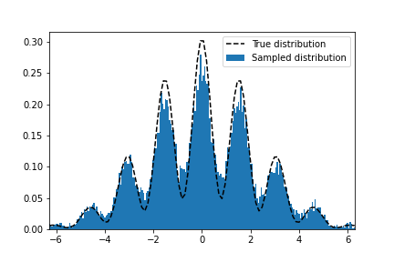
I’m not gonna lie though, this example was cherry-picked. Properly sampling with Markov Chain Monte Carlo (MCMC) methods is a finely honed skill unto itself, but hopefully you can rest assured that this at least works in theory!
Training diffusion models
Deriving the loss function
We want the generative distribution p(x_t), to match the observed distribution, p_data(x), when t goes to infinity. However, since infinity is hard to deal with, let’s do something kind of strange but in line with the literature. Suppose that at time t=0, we have the desired distribution p(x, t=0) = p_data(x). Then, without loss of generality, we impose that at some time t=T in the future, we have sufficiently destroyed (diffused) our distribution so that p(x, t=0) = N(x |0, 1). Finally, we need a loss that will push the observed and parametrized distributions closer to each other. We can do so by minimizing their KL-divergence, which gives us the seemingly simple objective L = — ∫p_data(x_0) ln p(x_0; 𝜗) dx_0.
As usual, p_data is non-integrable (we don’t know it, but we do have sample from it, i.e. the dataset). This is overcome in the usual way by replacing the integral with a summation over random mini-batches of the observed dataset (integration <=> summation swap-a-roo). The log-term is the difficult one. Using our fully expanded Markov form, with all the annoying integrals that it brings along, we can write it like this:

From here, we need to remove the integrals and simplify until we have something that we can code up. Doing so is a slog, so I’m just going to outline the main insights you need. The full derivation can be found in the accompanying notes.
Removing integrals with importance sampling
First we need to take care of those pesky integrals. To do so, we’ll use an age-old trick: importance sampling. If you have some integral like ∫ f(x) dx that’s giving you trouble, you can approximate it as the expectation E_{x ~ q(x)}[f(x)/q(x)] for some other distribution q(x). If you want to sound fancy though, you can say you got inspiration for this idea from annealed importance sampling and the Jarzynski equality. Let’s call the distribution q(x_0, …, x_T). Any distribution will do, but the question is, what do we pick? The answer is the least expensive one we can.
Humorous aside: I was once on a trip overseas, and thought it would be nice to bring home some bottles of wine from a local wineshop. At the time I was still a broke student, and needless to say I was experiencing some mild sticker shock. Overwhelmed, I gently walked over to the shopkeeper, and in a quiet voice politely asked what the cheapest bottles were. The next thing I know, the consternated shopkeeper’s eyes widen as she slams her palm on the table, and loudly reprimands, “We don’t sell cheap wine!” I’d like to point out, that being a student doesn’t just mean you’re broke, but also that you’re awkward. So my response to this blaring shopkeeper was to squint my eyes as if I were re-enacting the Futurama Fry meme, and respond, “Ok… but by definition, at least like one of these wines has to be the cheapest, right?” Perturbed, the shopkeeper proceeded to lift her hand from the table, turning her knuckles towards me and pinching with her thumb to her fingers. She then leaned forward, and in much calmer voice, explained to me, “Least expensive. Nothing cheap. I can sell you the least expensive wine.” To this day, I’ve made sure to never once ask for something cheap. I always ask for least expensive 🤌.
Here is where the diffusion part of diffusion models comes into play. A basic diffusion process is pretty much the simplest Markov distribution that we can construct for q(x_0, …, x_T) that admits an analytical expression. Let’s now assign names to our two distributions:
Forward (destructive/diffusive) process: q(x_0, …, x_T). This is the diffusion that we will analytically solve for to use in importance sampling.
Backward (generative) process: p(x_0, …, x_T). This is the thing that contains our learnable parameters and transition kernels, and will be used to generate samples.
The loss is now:

Use the Evidence Lower Bound (ELBO)
Trick #2 is another familiar trick (in this case approximation). Use Jensen’s inequality to optimize the ELBO instead. This means that you can move the logarithm past the integral and past q(x_1:T | x_0):

Making some cancellations and further simplifying, ultimately you’ll be able to express this in terms of KL divergences


This is the general form.
Turn the forward process into a diffusion process
Up until this point, we have not said anything about either the forward or backward processes, except that they are Markov. Let’s now sacrifice generality for the sake of tractability, and turn the forward process into a diffusion process. We’ll follow the method in the Denoising Diffusion Probabilistic Models (DDPM) paper, and make the following choice (Trick #3!) for the forward transition kernel

where the ⍺_t’s are fixed, time-dependent values. We can see that they are easily related to the noise variances at different times via variance β_t = 1 —⍺_t.
Choose larger variances at later times
Our choice of diffusion kernel might seem totally random, but it is actually very clever. Note that the diffusion process is defined by its variance, and here we are making a decision that the variances should be time-dependent. The previous schedule will miraculously make q(x_t | x_0) analytical in closed form (shown in the notes), and ensures that the variance does not explode over time.
I also want to make one important remark. Choosing progressively larger variances as the sample gets further and further away from p_data(x) is critical to the performance of diffusion models. Intuitively, you can think about it like this.
Suppose you’re far away from the center of the distribution. To you, it might look similar to how stars in the sky look — all shapes, bumps, and features are blurred into a single focused dot somewhere far in the distance. At this stage, it makes sense to take large leaps until you get close enough to resolve distances better, and only then decrease the size of your leaps. Otherwise, you’ll spend a lot of time optimizing for random things that have nothing to do with the correct direction to travel in space.
Define the backward (generative) kernel to be Gaussian
Believe it or not, the generative process has still been general up until this point. If you read the Physics aside, the motivation for this next step should hopefully be clear. If not, just think of it as an easy choice. We will parameterize the backward kernel via a normal distribution with learnable mean and fixed variance: p(x_t | x_{t-1}) = N(μ(x, t; 𝜗), β(t)). This will convert a lot of integrals into KL-divergences between two Gaussians, and in general, make much of the math simpler. Ultimately, you’ll find that the total loss is a sum of the losses for each possible timestep, and each loss has the same form. The result is:

where L_{t-1} is the loss for the (t-1)th timestep, The final step involves rewriting this in terms of just the noise ϵ, so that we get:

The μ term is only important to remember when it comes time to sample.
The final result, a de-noising objective
The loss expression is incredibly simple, and also intuitive. It says that at any given time step, there is some amount of Gaussian noise that was applied to the input, and our task is to predict it (hence de-noising). This suggests the following simplification, which in practice turns out to be more performant: drop the coefficient in the loss function. We’ve finally reached the diffusion algorithm. Here, I’ll copy/paste the algorithm from the original paper instead of retyping it
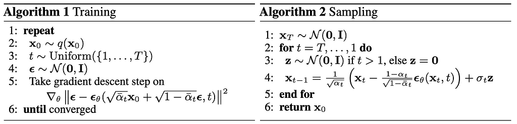
The σ_t are just the standard deviations, and given by √(1-⍺_t) (honestly don’t know why they couldn’t just write that 🤷♂️).
Sampling
I brushed over this one, but sampling is pretty straightforward to derive since we have normal distributions. The above derivation came from the reparametrization trick, namely, one can sample from x ~ N(µ, σ) by first sampling z ~ N(0, 1), then computing x = µ + σ z. By beginning our sampling at x_T, then sampling backward, we see that x_{T-1} ~ p(x_{T-1} | x_T) is easily sampled, which implies x_{T-2} ~ p(x_{T-2} | x_{T-1}) is easily sampled and so on. This also goes under the name ancestral sampling, which encompasses more complicated graph conditional dependencies as well.
For completeness, if you look at step (4) in Algorithm 2, notice that it has the form of a Langevin equation, as we discussed earlier.
Troubleshooting
The problem of bad inputs
When I first read the final DDPM algorithm, I was honestly pretty shocked that it works at all. Why would our model be able to get any information out of undoing some random Gaussian noise applied to it? How would this even work when our datapoint x is far from the center of the distribution? How can we learn dynamics when we’re literally just given a single snapshot in time?
For the first question, the answer is that if you look at Eq. (5) in the training algorithm, we’re actually feeding the noise into the model. The key point here, is that we are also feeding in the time. That additional bit of information seems to make the difference. My guess is that it allows the model reason about how close to the true distribution it is, and use that to better filter noise.
For the third question, I think the answer is ensembling. If the equilibrium distribution were known, it would be simple to write down the Fokker-Planck equation. That’s kind of what they were initially designed for anyway. In general, we can determine equilibrium by either (a) simulating some particles for a loooong time or (b) simulating a looooot of particles for a shorter time. As you get more and more data, I think you get closer to option (b) which is why this works.
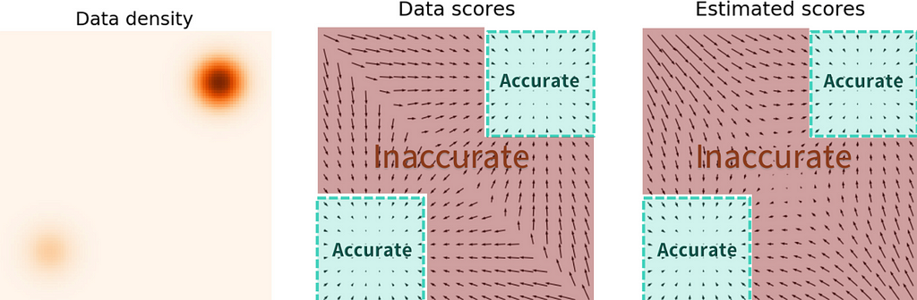
For the second question, the answer is that it doesn’t. lol. I’m not going to do disservice to the OG author who studied this, so I defer to his own blog about this. Under the section header “Naive score-based generative modeling and its pitfalls”, you’ll find the gist. The short story is that low-density regions get totally screwed in the loss function. Here is a visual of what this would look like for learning the flow of two Gaussians in the lower-left and upper-right corners:
I think this problem gets remedied somewhat for Poisson flow models, since those are biased to reproduce a monopole field. But, I don’t have the proof to back that up.
High variances
The worst feeling is watching your diffusion model slowly get closer and closer to a reasonably good image, only to yell skrt skrrrrtttt and swerve at the last moment into what looks like a TV from the 90s tuned to channel 100. There is a tradeoff between step size and variance. Smaller variances + more steps is always going to be a more accurate representation of the stochastic ODE, but it’s also more compute intensive. Make sure to pay attention here.
Coding
Getting these things to work in practice can actually be a bit annoying, mostly due to question (2) in the last section about low density regions. You’ll need to make sure that the prior distribution is sampled in a region that is able to be reached from the true target distribution via diffusion. Also, you’ll need to tune the number of diffusion steps and the variance schedule. Some other papers (cf. Improved Denoising Diffusion Probabilistic Models) set about optimizing these things, and found that replacing the fancy discrete variance schedules we derived with some simple 1D functions of time can do much better.
As far as coding this up, it’s actually startling easy. You’ll need:
- A model that takes as input a vector x and a time t, and returns another vector y of the same dimension as x. Specifically, the function looks something like y = model(x, t). Depending on your variance schedule, the dependence on time t can be either discrete (similar to token inputs in a transformer) or continuous. If it’s discrete, you can use the good-old fashioned transformer positional encodings (shameless self plug), and if it’s continuous, you can use Gaussian random features.
- A Mixin that handles all of the scheduling, sampling, and de-noising loss computation for a particular model.
To illustrate how this works, we’ll try to use a Diffusion model to learn a simple 2D spiral pattern. This was the toy dataset used in the original 2015 paper, so we’ll redo it using DDPM.
For an example scheduler, you can look at the DDPM class here. For convenience, I’m copy/pasting below:
import torch
from torch import nn


class DDPM(nn.Module):
    """Dataclass to maintain the noise schedule in the DDPM procedure of discrete noise steps
    Mathematically, the transition kernel at time $t$ is defined by:
    $$
    q(x_t|x_{t-1}) = \mathcal{N}(x_t| \sqrt{\alpha_t} x_{t-1}, 1 - \alpha_t)
    $$
    We further define quantities $\beta$ and $\bar \alpha$ in terms $\alpha$:
    $$
    \beta_t \equiv 1 - \alpha_t
    $$
    $$
    \bar \alpha_t = \prod_{t' < t}\alpha_{t'}
    $$
    which will be useful later on when computing transitions between non adjacent times.
    """

    def __init__(self, n_steps: int, minval: float = 1e-5, maxval: float = 5e-3):
        super().__init__()
        assert 0 < minval < maxval <= 1
        assert n_steps > 0
        self.n_steps = n_steps
        self.minval = minval
        self.maxval = maxval
        self.register_buffer("beta", torch.linspace(minval, maxval, n_steps))
        self.register_buffer("alpha", 1 - self.beta)
        self.register_buffer("alpha_bar", self.alpha.cumprod(0))

    def diffusion_loss(self, model: nn.Module, inp: torch.Tensor) -> torch.Tensor:
        device = inp.device
        batch_size = inp.shape[0]

        # create the noise perturbation
        eps = torch.randn_like(inp, device=device)

        # convert discrete time into a positional encoding embedding
        t = torch.randint(0, self.n_steps, (batch_size,), device=device)

        # compute the closed form sample x_noisy after t time steps
        a_t = self.alpha_bar[t][:, None]
        x_noisy = torch.sqrt(a_t) * inp + torch.sqrt(1 - a_t) * eps

        # predict the noise added given time t
        eps_pred = model(x_noisy, t)

        # Gaussian posterior, i.e. learn the Gaussian kernel.
        return nn.MSELoss()(eps_pred, eps)

    def sample(self, model: nn.Module, n_samples: int = 128):
        with torch.no_grad():
            device = next(model.parameters()).device

            # start off with an intial random ensemble of particles
            x = torch.randn(n_samples, 2, device=device)

            # the number of steps is fixed before beginning training. unfortunately.
            for t in reversed(range(self.n_steps)):
                # apply the same variance to all particles in the ensemble equally.
                a = self.alpha[t].repeat(n_samples)[:, None]
                abar = self.alpha_bar[t].repeat(n_samples)[:, None]

                # deterministic trajectory. eps_theta is similar to the Force on the particle
                eps_theta = model(x, torch.tensor([t] * n_samples, dtype=torch.long))
                x_mean = (x - eps_theta * (1 - a) / torch.sqrt(1 - abar)) / torch.sqrt(
                    a
                )
                sigma_t = torch.sqrt(1 - self.alpha[t])

                # sample a different realization of noise for each particle and propagate
                z = torch.randn_like(x)
                x = x_mean + sigma_t * z

            return x_mean  # clever way to skip the last noise addition
For some sample models in the case of both discrete and continuous time, you can check out the code here.
The training procedure is pretty much identical to a normal training procedure, except there are no targets in your batches and you’ll have to use the diffusion_loss method from the DDPM scheduler to compute the loss. You can find the training loop in the main.py script of the DDPM package.
If training is successful, you’ll find that the generated distributions look something like this:
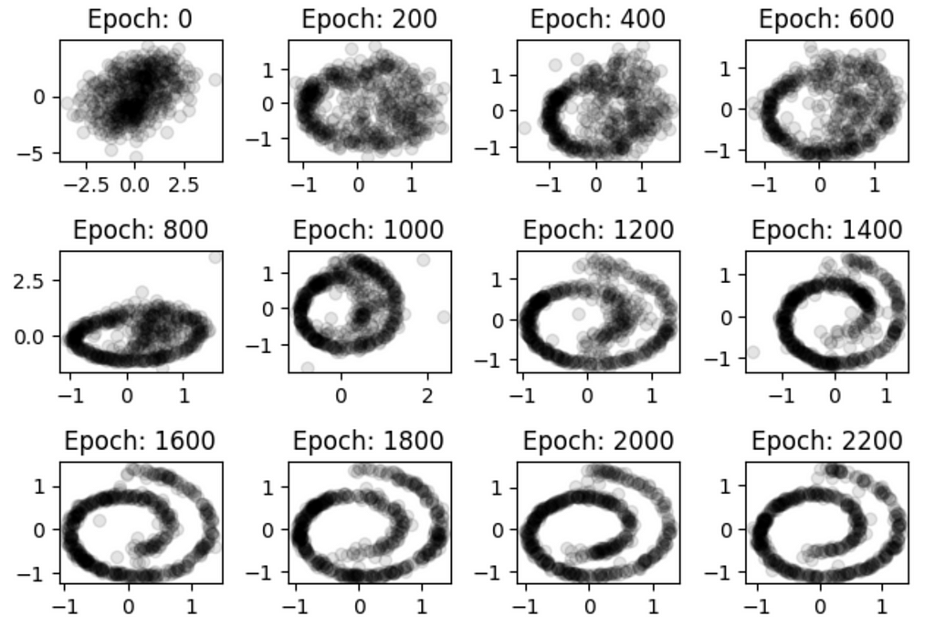
progressing from a random gaussian blob, to a neat, ordered spiral.
Wrapping things up
Things in the diffusion space have moved extremely quickly in the last couple of years, and for good reason. The results of some recent (2022) models like Dalle-2, StableDiffusion, and Midjourney have been astonishing to say the least. Combined with the current fervor for Generative AI, you have new developments occurring at a rapid pace. As such, there are plenty of exciting things to explore beyond this article.
For one, I didn’t mention any of the popular text-to-image models out there. These are large, complicated, multi-modal architectures that are many GPUs beyond the scope of this post. Other avenues for further study could include better methods for actually training diffusion models. I only briefly mentioned that there have been some studies into optimizing these, but of course there’s much deeper you can go. Another interesting avenue is to look at conditioned models. Some of the papers I mentioned also touched on this, but I didn’t want to go too far afield. There has been a lot of interesting work on guiding these diffusion models towards particular outcomes, whether it be class conditioning or otherwise. Other areas of study look at the tradeoffs between novelty and fidelity, as well as how to adjust the outputs in other ways like by negative sampling.
For me, the biggest question I wanted answered before beginning this blog post was, “How do these things actually work, and why?” I hope this post has at least given some partially satisfying answers 😄!
Diffusion models was originally published in Towards Data Science on Medium, where people are continuing the conversation by highlighting and responding to this story.
...