

 800+ IT
News
als RSS Feed abonnieren
800+ IT
News
als RSS Feed abonnieren📚 Fighting doppelgängers
💡 Newskategorie: AI Nachrichten
🔗 Quelle: towardsdatascience.com
How to rid data of evil twins reducing the feature space

Abstract
Given a large data set including many variables, some of these could represent the same phenomenon, or bring overlapping information to each other. A common pre-processing strategy to face this problem is to analyze correlations. In this article, I describe a strategy for scanning a network of linear correlations, searching for the best variable to keep, and dropping the redundant ones. Further, I present an R package to easily perform this job.
When working with data produced by sensors recording machinery events, large datasets including hundreds or thousands of variables are usual. In these cases, many variables can be candidates to predict some target measures. However, especially in industrial contexts, data can include fully linearly dependent or very correlated variables.
For example, a sensor can extract several features from the same process as linear transformations of the same basis (like the sum of a set of records, their mean, etc.). In other cases, there are genuinely different measures but related by nature, or representing two opposite facets of the same phenomenon (imagine two complementary elements of a chemical mixture).
Very correlated variables are redundant, and often they do not bring additional information. Moreover, fully dependent variables crash some machine learning algorithms. In general, these “doppelgängers” complicate the model-building process, adding computational weight and producing overfitting in some cases.
So, the question is: how to prune a data set to get rid of wicked doppelgängers?
Setting a threshold for correlation
A powerful weapon at our disposal to identify duplicated or nearly-duplicated variables is the linear correlation index.
When the correlation between two variables is ~|1|, retaining one or the other variable is irrelevant from a purely statistical point of view.
The situation gets complicated when the correlation is lower than |1|, but still relevant, and a theoretical-based choice is impractical. In these cases, we need a criterion for determining whether a correlation is relevant or not. One strategy is to set a threshold on the correlation value.
Given a threshold, we can focus on strong relations to implement a pruning strategy.
Pruning strategies
The key idea of pruning is dropping the most possible number of variables and retaining the greatest possible amount of information.
Imagine a situation where three variables, A, B, and C, have a strong relation. B has an over-threshold correlation both with A and C, while A and C have with each other an under-threshold correlation. The image below resumes these relations, representing each variable as a node of a network, and connecting two variables if their correlation is above the established threshold.
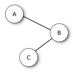
In the face of this situation, a pruning approach can be dropping B, retaining the lowly correlated A and C. However, a more parsimonious approach exists: retaining only B, dropping A and C. B can be considered the representative of the network and it can work as a spokesperson for the entire community.
As you can see, therefore, the choice is not unique.
To better understand the differences between these two approaches, I introduce a data set with more complex relations.
A more sophisticated example
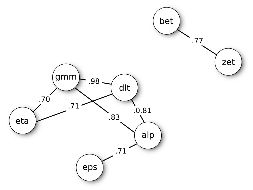
The image below is the network correlation obtained from seven simulated variables (alpha, beta, gamma, delta, epsilon, zeta, eta). The variables are spatially distributed in the graph according to the strength of their relation: near variables are more correlated to each other. Only relations above the threshold |0.7| are represented.
Source data are available in the data frame measures included in my R package doppelganger.
I build the graph above by hand, but if you are an R user, consider using the package qgraph to visualize a correlation matrix as a network. If you are a Python user, I suggest taking a look at this article on TDS. From this point forward, I use the R language to build examples.
I report below the full correlation matrix.
r <- cor(doppelganger::measures)
diag(r) <- NA
round(r, 3)
        alpha  beta gamma delta epsilon  zeta   eta
alpha      NA 0.129 0.833 0.815   0.715 0.207 0.645
beta    0.129    NA 0.152 0.108   0.056 0.770 0.097
gamma   0.833 0.152    NA 0.984   0.620 0.193 0.702
delta   0.815 0.108 0.984    NA   0.588 0.167 0.711
epsilon 0.715 0.056 0.620 0.588      NA 0.072 0.519
zeta    0.207 0.770 0.193 0.167   0.072    NA 0.137
eta     0.645 0.097 0.702 0.711   0.519 0.137    NA
The graph shows the presence of two communities: one for the pair zeta-beta, and another one including the remaining variables. The situation is messier when compared to the previous naive example. How to proceed?
Prioritizing variables
We can rank variables according to their centrality degree, intended as the strength of the connections of a node with other nodes. The most central nodes correspond to the most representative variables of the network.
We can calculate the centrality degree as the mean of absolute values of the correlations referring to a variable. The R code below calculates the centrality of each node and sorts them in decreasing order.
sort(colMeans(abs(r), na.rm=TRUE), decreasing=TRUE)
    gamma     delta     alpha       eta   epsilon      zeta      beta
0.5805754 0.5620824 0.5572697 0.4685961 0.4282394 0.2575334 0.2188217
The ranking by centrality degree allows us to prioritize variables when choosing what to keep and what to drop. We have two ways before us:
- to keep the most central variables, in the name of their representativeness (centrality criterion);
- to keep the most peripheral variables, in the name of their independence (peripherality criterion).
Anyway, we can apply the same pruning procedure, but:
in the “centrality” case we scan the variables following the centrality degree vector in decreasing order, while in the “peripherality” case we follow the increasing order.
We start keeping the first variable in the ranking, dropping its doppelgängers. Afterward, let’s keep the second variable, dropping its doppelgängers. Et so on, until the end. Simple, isn’t it?
Algorithm application
Now, apply the procedure to the example shown above. I describe the operations following the centrality criterion.
STEP 1. The most central variable is gamma. So, we “turn on” gamma and “turn off” delta, alpha, and eta, which have with gamma an over-threshold correlation. In the image below, the “turned off” variables are marked in light gray, and their corrections are dashed.
STEP 2. After gamma, following the priority order, the first non-dropped variable is epsilon. However, epsilon hasn’t over-threshold correlations with the remaining variables. Its doppelgängers are already dropped, so no action is required.
STEP 3. The following variable is zeta, which has a strong correlation with beta. So, we drop beta, retaining zeta.
At the end of iterations, we will remain with gamma, epsilon, and zeta. Three variables instead of seven.
Centrality versus peripherality
The centrality criterion takes advantage of the presence of isolated communities within the population of variables. From a theoretical perspective, this method gives its best when we have strong connections within communities and weak connections between communities. The peripherality criterion, on the opposite, can give its best with more homogeneous networks including a few subgroups.
The centrality criterion tends to keep less but more correlated variables. The peripherality criterion tends to keep more variables but less correlated, however, they not necessarily are the most representative of each subgroup.
The doppelganger package for R
The previous steps can be performed by only one line of code using the R package doppelganger.
Loading the package and the data set :
library(doppelganger)
measures # comes with the package

# A tibble: 100 × 7
     alpha     beta   gamma  delta epsilon    zeta     eta
     <dbl>    <dbl>   <dbl>  <dbl>   <dbl>   <dbl>   <dbl>
 1  0.0185 -0.564   -0.526  -0.368  -0.934 -0.878   0.0913
 2  0.120   0.00233 -0.414  -0.515  -0.193 -0.464  -0.324
 3 -0.767   0.0641  -1.51   -1.26   -1.25  -0.0825 -1.70
 4 -2.12    0.105   -2.38   -2.37   -1.75  -0.323  -0.426
 5 -1.48   -0.126   -0.681  -0.340  -1.87   0.0678 -0.791
 6  1.69    0.268    2.39    2.59    1.06   0.115   1.44
 7  1.26   -1.17     0.290   0.231   1.93  -0.683  -0.253
 8  1.23    1.40     1.10    0.997   0.717  1.07    0.265
 9  0.295  -0.0263  -0.0221 -0.115  -0.125  0.179  -0.978
10  0.157   0.268    0.215   0.454   0.531  1.25   -0.0989
# … with 90 more rows
Reproducing the pruning process of variables described above:
dg <- doppelganger(measures, priority="c", threshold=0.7)
The homonymous function doppelganger creates a list object containing some slots, including keep and drop, collecting the names of variables respectively to keep and to drop.
dg$keep

[1] "gamma"   "epsilon" "zeta"
If you need to inspect correlations of a specific variable, the package makes available the function inspect_corrs:
inspect_corrs(dg, "gamma")

# A tibble: 6 × 3
  variable is_alias   cor
  <chr>    <lgl>    <dbl>
1 delta    TRUE     0.984
2 alpha    TRUE     0.833
3 eta      TRUE     0.702
4 epsilon  FALSE    0.620
5 zeta     FALSE    0.193
6 beta     FALSE    0.152
Weighting for non-missing data
The package doppelganger calculates the centrality degree by weighting each correlation with the number of observations available for the calculus of the index. This strategy is effective in presence of missing data because it allows “rewarding” variables with many filled records matching filled records of other variables.
We desire to retain the best variables, but also retain the greatest possible number of records!
The pruning of a pool of candidate predictors can be an effective ally in building a light and efficient model, especially for inferential purposes. The best practice is to base a selection procedure on theoretical assumptions or predictive capabilities of potential predictors. However, often, because lack of information or a dimension of the data set, this is impractical. In these cases, a less refined approach — like the one described in this post — can come in handy.
Fighting doppelgängers was originally published in Towards Data Science on Medium, where people are continuing the conversation by highlighting and responding to this story.
...