

 800+ IT
News
als RSS Feed abonnieren
800+ IT
News
als RSS Feed abonnieren📚 5 Data Similarity Metrics
💡 Newskategorie: AI Nachrichten
🔗 Quelle: towardsdatascience.com

Understanding Similarity Metrics in Data Analysis and Machine Learning: A Comprehensive Guide
Preface: This article presents a summary of information about the given topic. It should not be considered original research. The information and code included in this article have may be influenced by things I have read or seen in the past from various online articles, research papers, books, and open-source code.
Introduction
Similarity metrics are a vital tool in many data analysis and machine learning tasks, allowing us to compare and evaluate the similarity between different pieces of data. Many different metrics are available, each with pros and cons and suitable for different data types and tasks.
This article will explore some of the most common similarity metrics and compare their strengths and weaknesses. By understanding the characteristics and limitations of these metrics, we can choose the most appropriate one for our specific needs and ensure the accuracy and relevance of our results.
- Euclidean Distance
This metric calculates the straight-line distance between two points in n-dimensional space. It is often used for continuous numerical data and is easy to understand and implement. However, it can be sensitive to outliers and does not account for the relative importance of different features.
from scipy.spatial import distance

# Calculate Euclidean distance between two points
point1 = [1, 2, 3]
point2 = [4, 5, 6]

# Use the euclidean function from scipy's distance module to calculate the Euclidean distance
euclidean_distance = distance.euclidean(point1, point2)
- Manhattan Distance
This metric calculates the distance between two points by considering the absolute differences of their coordinates in each dimension and summing them. It is less sensitive to outliers than Euclidean distance, but it may not accurately reflect the actual distance between points in some cases.
from scipy.spatial import distance

# Calculate Manhattan distance between two points
point1 = [1, 2, 3]
point2 = [4, 5, 6]

# Use the cityblock function from scipy's distance module to calculate the Manhattan distance
manhattan_distance = distance.cityblock(point1, point2)

# Print the result
print("Manhattan Distance between the given two points: " + \
      str(manhattan_distance))
- Cosine Similarity
This metric calculates the similarity between two vectors by considering their angle. It is often used for text data and is resistant to changes in the magnitude of the vectors. However, it does not consider the relative importance of different features.
from sklearn.metrics.pairwise import cosine_similarity

# Calculate cosine similarity between two vectors
vector1 = [1, 2, 3]
vector2 = [4, 5, 6]

# Use the cosine_similarity function from scikit-learn to calculate the similarity
cosine_sim = cosine_similarity([vector1], [vector2])[0][0]

# Print the result
print("Cosine Similarity between the given two vectors: " + \
      str(cosine_sim))Jaccard Similarity
- Jaccard Similarity
This metric calculates the similarity between two sets by considering the size of their intersection and union. It is often used for categorical data and is resistant to changes in the size of the sets. However, it does not consider the sets' order or frequency of elements.
def jaccard_similarity(list1, list2):
    """
    Calculates the Jaccard similarity between two lists.

    Parameters:
    list1 (list): The first list to compare.
    list2 (list): The second list to compare.

    Returns:
    float: The Jaccard similarity between the two lists.
    """
    # Convert the lists to sets for easier comparison
    s1 = set(list1)
    s2 = set(list2)

    # Calculate the Jaccard similarity by taking the length of the intersection of the sets
    # and dividing it by the length of the union of the sets
    return float(len(s1.intersection(s2)) / len(s1.union(s2)))

# Calculate Jaccard similarity between two sets
set1 = [1, 2, 3]
set2 = [2, 3, 4]
jaccard_sim = jaccard_similarity(set1, set2)

# Print the result
print("Jaccard Similarity between the given two sets: " + \
      str(jaccard_sim))
- Pearson Correlation Coefficient
This metric calculates the linear correlation between two variables. It is often used for continuous numerical data and considers the relative importance of different features. However, it may not accurately reflect non-linear relationships.
import numpy as np

# Calculate Pearson correlation coefficient between two variables
x = [1, 2, 3, 4]
y = [2, 3, 4, 5]

# Numpy corrcoef function to calculate the Pearson correlation coefficient and p-value
pearson_corr = np.corrcoef(x, y)[0][1]

# Print the result
print("Pearson Correlation between the given two variables: " + \
      str(pearson_corr))
Now that we have reviewed the basics of these distance metrics, let’s consider a practical scenario and apply them to compare the results.
Scenario
Suppose we have 5 items with numerical attributes and we want to compare the similarities between these products in order to facilitate applications such as clustering, classification, or perhaps, recommendations.
The following code computes the similarity metrics for the given products and their attributes using various distance metrics and then plots the results in a heat map for evaluation.
import numpy as np
import seaborn as sns
import random
import matplotlib.pyplot as plt
import pprint

def calculate_similarities(products):
    """Calculate the similarity measures between all pairs of products.

    Parameters
    ----------
    products : list
        A list of dictionaries containing the attributes of the products.

    Returns
    -------
    euclidean_similarities : numpy array
        An array containing the Euclidean distance between each pair of products.
    manhattan_distances : numpy array
        An array containing the Manhattan distance between each pair of products.
    cosine_similarities : numpy array
        An array containing the cosine similarity between each pair of products.
    jaccard_similarities : numpy array
        An array containing the Jaccard index between each pair of products.
    pearson_similarities : numpy array
        An array containing the Pearson correlation coefficient between each pair of products.
    """
    # Initialize arrays to store the similarity measures
    euclidean_similarities = np.zeros((len(products), len(products)))
    manhattan_distances = np.zeros((len(products), len(products)))
    cosine_similarities = np.zeros((len(products), len(products)))
    jaccard_similarities = np.zeros((len(products), len(products)))
    pearson_similarities = np.zeros((len(products), len(products)))

    # Calculate all the similarity measures in a single loop
    for i in range(len(products)):
        for j in range(i+1, len(products)):
            p1 = products[i]['attributes']
            p2 = products[j]['attributes']

            # Calculate Euclidean distance
            euclidean_similarities[i][j] = distance.euclidean(p1, p2)
            euclidean_similarities[j][i] = euclidean_similarities[i][j]

            # Calculate Manhattan distance
            manhattan_distances[i][j] = distance.cityblock(p1, p2)
            manhattan_distances[j][i] = manhattan_distances[i][j]

            # Calculate cosine similarity
            cosine_similarities[i][j] = cosine_similarity([p1], [p2])[0][0]
            cosine_similarities[j][i] = cosine_similarities[i][j]

            # Calculate Jaccard index
            jaccard_similarities[i][j] = jaccard_similarity(p1, p2)
            jaccard_similarities[j][i] = jaccard_similarities[i][j]

            # Calculate Pearson correlation coefficient
            pearson_similarities[i][j] = np.corrcoef(p1, p2)[0][1]
            pearson_similarities[j][i] = pearson_similarities[i][j]

    return euclidean_similarities, manhattan_distances, cosine_similarities, jaccard_similarities, pearson_similarities

def plot_similarities(similarities_list, labels, titles):
    """Plot the given similarities as heatmaps in subplots.

    Parameters
    ----------
    similarities_list : list of numpy arrays
        A list of arrays containing the similarities between the products.
    labels : list
        A list of strings containing the labels for the products.
    titles : list
        A list of strings containing the titles for each plot.

    Returns
    -------
    None
        This function does not return any values. It only plots the heatmaps.
    """
    # Set up the plot
    fig, ax = plt.subplots(nrows=1,
                           ncols=len(similarities_list), figsize=(6*len(similarities_list), 6/1.680))

    for i, similarities in enumerate(similarities_list):
        # Plot the heatmap
        sns.heatmap(similarities, xticklabels=labels, yticklabels=labels, ax=ax[i])
        ax[i].set_title(titles[i])
        ax[i].set_xlabel("Product")
        ax[i].set_ylabel("Product")

    # Show the plot
    plt.show()

# Define the products and their attributes
products = [
    {'name': 'Product 1', 'attributes': random.sample(range(1, 11), 5)},
    {'name': 'Product 2', 'attributes': random.sample(range(1, 11), 5)},
    {'name': 'Product 3', 'attributes': random.sample(range(1, 11), 5)},
    {'name': 'Product 4', 'attributes': random.sample(range(1, 11), 5)},
    {'name': 'Product 5', 'attributes': random.sample(range(1, 11), 5)}
]

pprint.pprint(products)

euclidean_similarities, manhattan_distances, \
cosine_similarities, jaccard_similarities, \
pearson_similarities = calculate_similarities(products)

# Set the labels for the x-axis and y-axis
product_labels = [product['name'] for product in products]

# List of similarity measures and their titles
similarities_list = [euclidean_similarities, cosine_similarities, pearson_similarities,
                     jaccard_similarities, manhattan_distances]
titles = ["Euclidean Distance", "Cosine Similarity", "Pearson Correlation Coefficient",
          "Jaccard Index", "Manhattan Distance"]

# Plot the heatmaps
plot_similarities(similarities_list, product_labels, titles)
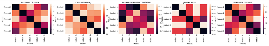
As we can see from the charts, each similarity metric produces a heat map that represents different similarities between the products, and on a different scale. While each similarity metric can be used to interpret whether two products are similar or not based on the metric’s value, it is difficult to determine a true measure of similarity when comparing the results across different distance metrics.
How to correct metric?
There is no single “true” answer when it comes to choosing a similarity metric, as different metrics are better suited for different types of data and different analysis goals. However, there are some factors that can help narrow down the possible metrics that might be appropriate for a given situation. Some things to consider when choosing a similarity metric include:
- The type of data: Some metrics are more appropriate for continuous data, while others are better suited for categorical or binary data.
- The characteristics of the data: Different metrics are sensitive to different aspects of the data, such as the magnitudes of differences between attributes or the angles between attributes. Consider which characteristics of the data are most important to your analysis and choose a similarity metric that is sensitive to these characteristics.
- The goals of your analysis: Different metrics can highlight different patterns or relationships in the data, so consider what you are trying to learn from your analysis and choose a distance metric that is well-suited to this purpose.
Personally, I often use the following chart as a starting point when choosing a similarity metric.
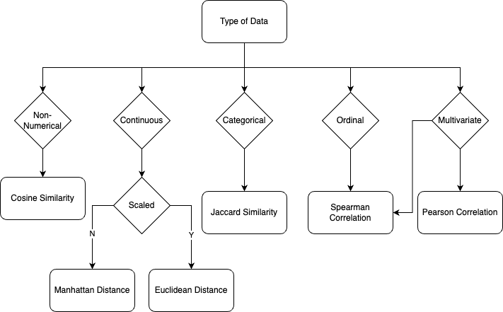
Again, it is important to carefully consider the data type and characteristics when selecting a similarity metric, as well as the specific goals of the analysis.
All of the code used in this article can be found at Jupyter Notebook.
Thanks for reading. If you have any feedback, please feel to reach out by commenting on this post, messaging me on LinkedIn, or shooting me an email (shmkapadia[at]gmail[dot]com)
If you liked this article, read my other articles
5 Data Similarity Metrics was originally published in Towards Data Science on Medium, where people are continuing the conversation by highlighting and responding to this story.
...