

 800+ IT
News
als RSS Feed abonnieren
800+ IT
News
als RSS Feed abonnieren📚 Implementing Word2vec in PyTorch from the Ground Up
💡 Newskategorie: AI Nachrichten
🔗 Quelle: towardsdatascience.com
A Step-by-Step Guide to training a Word2vec Model

Introduction
An important component of natural language processing (NLP) is the ability to translate words, phrases, or larger bodies of text into continuous numerical vectors. There are many techniques for accomplishing this task, but in this post we will focus in on a technique published in 2013 called word2vec.
Word2vec is an algorithm published by Mikolov et al. in a paper titled Efficient Estimation of Word Representations in Vector Space. This paper is worth reading, though I will provide an overview as we build it from the ground up in PyTorch. Succinctly, word2vec uses a single hidden layer artificial neural network to learn dense word embeddings. These word embeddings allow us to identify words that have similar semantic meanings. Additionally, word embeddings allow us to apply algebraic operations. For example “vector(‘King’) - vector(‘Man’) + vector(‘Woman’) results in a vector that is closest to the vector representation of the word Queen” (“Efficient Estimation of Word Representations in Vector Space” 2).
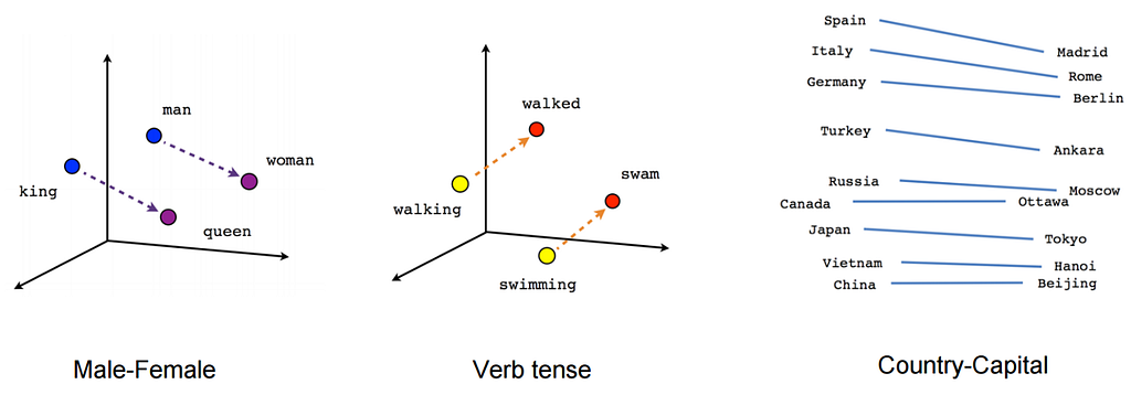
Figure 1 is an example of word embeddings in 3-dimensions. Word embeddings can learn semantic relationships between words. The “Male-Female” example illustrates how the relationship between “man” and “woman” is very similar to the relationship between “king” and “queen.” Syntactic relationships can be encoded by embeddings as is shown in the “Verb tense” example.
Word Embeddings Overview
Before we get into the model overview and PyTorch code, let’s start with an explanation of word embeddings.
Why do we even need word embeddings?
Computers are simply abstracted calculators. They are really efficient at doing mathematical computations. Any time we want to express our thoughts to a computer, the language we must use is numerical. If we want to figure out the sentiment of a yelp review or the topic of a popular book, we will need to first translate the text into vectors. Only then can we use follow-on procedures to extract the information of interest from the text.
Simplest word embeddings
Word embeddings are precisely how we translate our thoughts into a language computers can understand. Let’s work through an example taken from the Wikipedia article on python that states “python consistently ranks as one of the most popular programming languages.” This sentence contains 11 words, so why don’t we create a vector of length 11 where each index takes the value 1 if the word is present and a 0 if it is not? This is commonly known as one-hot encoding.
python       = [1,0,0,0,0,0,0,0,0,0,0]
consistently = [0,1,0,0,0,0,0,0,0,0,0]
ranks        = [0,0,1,0,0,0,0,0,0,0,0]
as           = [0,0,0,1,0,0,0,0,0,0,0]
one          = [0,0,0,0,1,0,0,0,0,0,0]
of           = [0,0,0,0,0,1,0,0,0,0,0]
the          = [0,0,0,0,0,0,1,0,0,0,0]
most         = [0,0,0,0,0,0,0,1,0,0,0]
popular      = [0,0,0,0,0,0,0,0,1,0,0]
programming  = [0,0,0,0,0,0,0,0,0,1,0]
languages    = [0,0,0,0,0,0,0,0,0,0,1]
This method of converting words into vectors is arguably the simplest. Yet, there are a few shortcomings that will provide the motivation for word2vec embeddings. First, the length of the embedding vectors increases linearly with the size of the vocabulary. Once we need to embed millions of words, this method of embedding becomes problematic in terms of space complexity. Second is the issue that these vectors are sparse. Each vector has only a single entry with value 1 and all remaining entries have value 0. Once again, this is a significant waste of memory. Finally, each word vector is orthogonal to every other word vector. Therefore, there is no way to determine which words are most similar. I would argue that the words “python” and “programming” should be considered more similar to each other than “python” and “ranks.” Unfortunately, the vector representations for each of these words is equally different from every other vector.
Improved Word Embeddings
Our goal is now more refined: can we create fixed-length embeddings that allow us to identify which words are most similar to each other? An example might be:
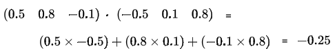
python       = [0.5,0.8,-0.1]
ranks        = [-0.5,0.1,0.8]
programming  = [0.9,0.4,0.1]
If we take the dot product of “python” and “ranks”, we would get:
And if we take the dot product of “python” and “programming”, we would get:
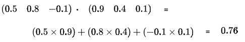
Since the score between “python” and “ranks” is lower than that of “python” and “programming”, we would say that “python” and “programming” are more similar. Generally, we will not use the dot product between two embeddings to compute a similarity score. Instead, we will use the cosine similarity since it removes the effect of vector norms and returns a more standardized score. Regardless, Both of the issues we faced with the one-hot encoding method are solved — our embedding vectors are of fixed length and they allow us to compute similarity between words.
Skipgram Word2Vec architecture
Now that we have a grasp of word embeddings, the question becomes how to learn these embeddings. This is where Mikolov’s word2vec model comes into play. If you are unfamiliar with artificial neural networks, the following sections will be unclear since word2vec is fundamentally based on this type of model. I highly recommend checking out Michael Nielsen’s free online Deep Learning and Neural Networks course and 3Blue1Brown’s YouTube series on neural networks if this material is new for you.
Skipgrams
Recall the sentence from earlier, “python consistently ranks as one of the most popular programming languages.” Imagine someone didn’t know the word “programming” and wanted to figure out its meaning. A reasonable approach is to check the neighboring words for a clue about the meaning of this unknown word. They would notice that it was surrounded by “popular” and “language.” These words could give them a hint to the possible meaning of “programming”. This is precisely how the skipgram model works. Ultimately, we will train a neural network to predict the neighboring context words, given an input word. In Figure 2, the green word is the unknown target word and the blue words surrounding it are the context words our neural network will be trained to predict.
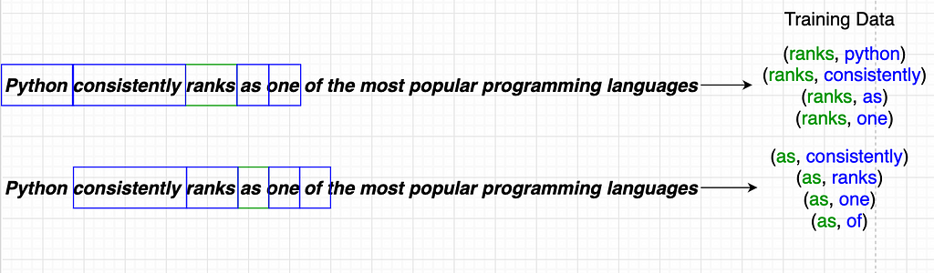
In this example, the window size is 2. This means that every target word will be surrounded by 2 context words that the model will need to predict. Since the word “rank” has 2 words to the left and 2 words to the right, the resulting training data is 4 examples for this target word.
Model Architecture
The neural network used to learn these word embeddings is a single hidden layer feedforward network. The inputs to the network are the target words. The labels are the context words. The single hidden layer will be the dimension in which we choose to embed our words. For this example, we will use an embedding size of 300.
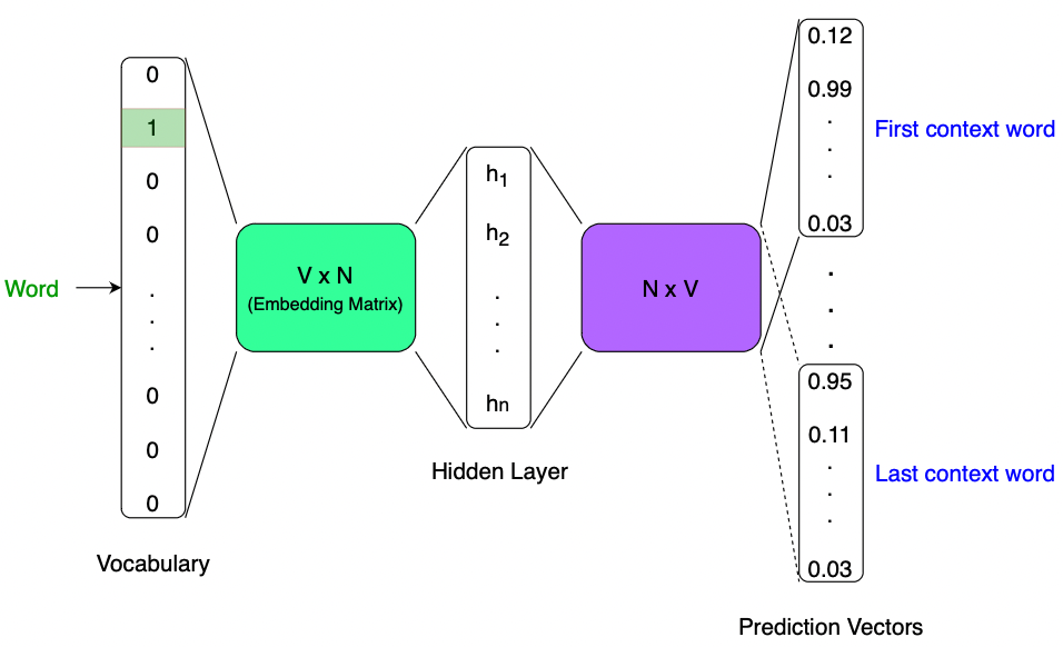
Let’s go through an example of how this model works. If we want to embed a word, the first step is to find its index in the vocabulary. This index is then passed to the networks as the row index in the embedding matrix. In Figure 3, the input word is the second entry in our vocabulary vector. This means that we will now will enter the green embedding matrix on the second row. This row is of length 300 — the embedding dimension, N. We then matrix multiply this vector, which is the hidden layer, by a second embedding matrix of shape N x V to result in a vector of length V.
Notice that there are Vcolumns in the second embedding matrix (the purple matrix). Each of these columns represents a word in the vocabulary. Another way to conceptualize this matrix multiplication is by recognizing that it results in the dot product between the vector for the target word (the hidden layer) and every word in the vocabulary (the columns of the purple matrix). The result is a vector of length V, representing the context word predictions. Since our context window size is 2, we will have 4 prediction vectors of length V. We then compare these prediction vectors with the corresponding ground truth vectors to compute the loss that we backpropagate through the network to update the model parameters. In this case, the model parameters are the elements of the embedding matrices. Discussion of the mechanics of this training procedure will be fleshed out in PyTorch code later on.
Negative Sampling

In the paper titled Distributed Representations of Words and Phrases and their Compositionality by Mikolov et al., the authors propose two enhancements to the original word2vec model — negative sampling and subsampling.
In Figure 3, notice how each prediction vector is of length V. The ground truth vectors that will be compared to each prediction vector will also be of length V, but the ground truth vectors will be extremely sparse since only a single element of the vector will be labeled 1 — the true context word the model is being trained to predict. This true context word will be referred to as the “positive context word”. Every other word in the vocabulary, which is V — 1 words, will be labeled 0 since they are not the context word in the training example. All of these words will be referred to as “negative context words”.
Mikolov et al. proposed a methodology called negative sampling that reduces the size of the ground truth vector and therefore the prediction vector. This reduces the computational requirements of the network and expedites training. Instead of using all the negative context words, Mikolov proposed a method to sample a small number of negative context words from the existingV — 1 negative context words using a conditional probability distribution.
In the code provided, I implement a negative sampling procedure that differs from the method Mikolov proposed. It was simpler to construct and still results in high-quality embeddings. In Mikolov’s paper, the probability that a negative sample is chosen is based on the conditional probability of seeing the candidate word in the context of the target word. So, for every word in the vocabulary, we would generate a probability distribution for every other word in the vocabulary. These distributions represent the conditional probability of seeing the other word in the target word’s context. Then, the negative context words would be sampled with a probability inversely proportional to the probability.
I implemented negative sampling in a slightly different way avoiding conditional distributions. First, I found the frequency of each word in the vocabulary. I ignored the conditional probability by finding the overall frequency. Then, an arbitrarily large negative sampling vector is populated with the vocabulary indices proportional to the frequency of the word. For example, if the word “is” comprises 0.01% of the corpus, and we decide the negative sampling vector should be of size 1,000,000, then 100 elements (0.01% x 1,000,000) of the negative sampling vector will be populated with the vocabulary index of the word “is”. Then, for every training example, we randomly sample a small number of elements from the negative sampling vector. If this small number is 20 and the vocabulary is 10,001 words, we just reduced the length of the prediction and ground truth vectors by 9,980 elements. This reduction speeds up the model training time substantially.
Subsampling
Subsampling is another method proposed by Mikolov et al. to reduce training time and improve model performance. The fundamental observation from which subsampling arises is that words with high frequency “provide less information value than the rare words” (“Distributed Representations of Words and Phrases and their Compositionality” 4). For instance, words like “is,” “the,” or “in” occur quite frequently. These words are highly likely to co-occur with many other words. This implies that the context words around these high-frequency words impart little contextual information about the high-frequency word itself. So, instead of using every word pair in the corpus, we sample the words with a probability inversely proportional to the frequency of the words in the pair. The exact implementation details will be explained in the following section.
PyTorch Implementation
With the overview of word embeddings, word2vec architecture, negative sampling, and subsampling out of the way, let’s dig into the code. Please note, there are frameworks that have abstracted away the implementation details of word2vec. These options are extremely powerful and provide the user extensibility. For example, gensim provides a word2vec API which includes additional functions such as using pretrained models and multi-word n-grams. However, in this tutorial we will create a word2vec model without leveraging any of these frameworks.
All the code we will review in this tutorial can be found on my GitHub. Please note, the code in the repository is subject to change as I work on it. For the purpose of this tutorial, a simplified version of this code will be presented here in a Google Colab notebook.
Getting Data
We will use a wikipedia dataset called WikiText103 provided by PyTorch for training our word2vec model. In the code below, you will see how I import and print the first few lines of the dataset. The first text comes from the wikipedia article on Valkyria Chronicles III.
https://medium.com/media/dbe34c1dda7029c6bd3fbe210b47eace/hrefSetting Parameters and Configuration
Now we will set parameters and configuration values that will be used throughout the rest of the code. Some of the parameters in this snippet are relevant to code later on in the notebook, but bear with me.
https://medium.com/media/19b0d49262297bcc35d72bbfa9c1baa9/hrefHere we construct a dataclass containing parameters that define our word2vec model. The first section controls text preprocessing and skipgram construction. We will only consider words that occur at least 50 times. This is controlled by the MIN_FREQ parameter. SKIPGRAM_N_WORDS is the window size we will consider for constructing the skipgrams. This means that we will look at 8 words before and after the target word. T controls the how we compute the subsampling probability. This means that words with frequency in the 85th percentile will have a small probability of being subsampled as we described in the subsampling section above. NEG_SAMPLES is the number of negative samples to use for each training example, as described in the negative sampling section above. NS_ARRAY_LEN is the length of the negative sampling vector that we will sample negative observations from. SPECIALS is the placeholder string for words that are excluded from the vocabulary if they do not meet the minimum frequency requirement. TOKENIZER refers to how we want to convert the corpus of text into tokens. The “basic_english” tokenizer splits all the text by spaces.
The second section defines the model configuration and hyperparameters. BATCH_SIZE is the number of documents that will be in each minibatch used to train the network. EMBED_DIMis the dimensionality of the embeddings we will use for every word in the vocabulary. EMBED_MAX_NORM is the maximum norm each embedding vector can be. N_EPOCHS is the number of epochs we will train the model for. DEVICE tells PyTorch whether to use a CPU or a GPU to train the model. CRITERION is the loss function used. Discussion of loss function choice will be continued when we discuss the model training procedure.
Building the Vocabulary
The next step in preparing the text data for our word2vec model is building a vocabulary. We will build a class called Vocab and it will have methods that allow us to lookup a word’s index and frequency. We will also be able to lookup a word by its index as well as get the total count of words in the entire corpus of text.
https://medium.com/media/b5afb72daebb5c3964bf2e081870dc39/hrefWithout reviewing every line in this code, note that the Vocab class has stoi, itos, and total_tokens attributes as well as get_index(), get_freq(), and lookup_token() methods. The following gist will show what these attributes and methods do.
https://medium.com/media/9accd2ca19c3b89754a819400f1ff3b0/hrefstoi is a dictionary where the keys are words and the values are the tuples of the index and the frequency of the key words. For example, the word “python” is the 13,898th most common word occurring 403 times. The entry in the stoi dictionary for this word would be {"python": (13898, 403)}. itos is similar to stoi, but its key is the index value such that the entry for “python” would be {13898: ("python", 403)}.The total_tokens attribute is the total number of tokens in the entire corpus. In our example there are 77,514,579 words.
The get_index() method takes a word or a list of words as an input and returns the index or the list of indices of these words. If we were to call Vocab.get_index("python") the returned value is 13898. The get_frequency() method takes a word or a list of words as an input and returns the frequency of the words as an integer or a list of integers. If we were to call Vocab.get_freq("python") the value returned is 403. Finally, the lookup_token() method takes an integer and returns the word that occupies that index. For example, if we were to call Vocab.lookup_token(13898), the method would return "python".
The final functions in the gist above are yield_tokens() and build_vocab()functions. The yield_tokens() function preprocesses and tokenizes the text. The preprocessing simply removes all characters that are not letters or digits. The build_vocab()function takes the raw wikipedia text, tokenizes it, and then constructs a Vocab object. Once again, I will not go over every line in this function. The key takeaway is that aVocab object is constructed by this function.
Building our PyTorch Dataloaders
The next step in the process is to construct the skipgrams with subsampling and then create dataloaders for our PyTorch model. For an overview on why dataloaders are so critical for PyTorch models that train on a lot of data, check out the documentation.
https://medium.com/media/0e252257fc77ae1754e2cf2167b7ad01/hrefThis class is probably the most complex we have worked on yet so let’s go through each method thoroughly starting with the last method, collate_skipgram(). We start by initializing two lists, batch_input and batch_output. Each of these lists will be populated with vocabulary indices. Ultimately, the batch_input list will have the indices for each target word and thebatch_output list will contain positive context word indices for each target word. The first step is to loop over every text in the batch and convert all the tokens to the corresponding vocabulary index:
for text in batch:
    text_tokens = self.vocab.get_index(self.tokenizer(text))
The next step checks to ensure the text is sufficiently long to generate training examples. Recall the sentence from earlier, “python consistently ranks as one of the most popular programming languages.” There are 11 words. If we set the SKIPGRAM_N_WORDS to be 8, then a document that is 11 words long is not sufficient since we cannot find a word in the document that has 8 context words before it as well as 8 context words after it.
if len(text_tokens) < self.params.SKIPGRAM_N_WORDS * 2 + 1:
    continue
Then we create a list of the target word and a list of all the context words surrounding the target word, ensuring that we always have a full set of context words:
for idx in range(len(text_tokens) - self.params.SKIPGRAM_N_WORDS*2):
    token_id_sequence = text_tokens[
        idx : (idx + self.params.SKIPGRAM_N_WORDS * 2 + 1)
        ]
    input_ = token_id_sequence.pop(self.params.SKIPGRAM_N_WORDS)
    outputs = token_id_sequence
Now, we implement subsampling. We lookup the probability that the target word is discarded given it’s frequency and then remove it with that probability. We will see how we compute these discard probabilities shortly.
prb = random.random()
del_pair = self.discard_probs.get(input_)
if input_==0 or del_pair >= prb:
    continue
Then, we execute the same subsampling procedure for the context words surrounding the target word, if the previous step did not remove the target word itself. Finally, we append the resulting data to the batch_input and batch_output lists, respectively.
else:
    for output in outputs:
        prb = random.random()
        del_pair = self.discard_probs.get(output)
        if output==0 or del_pair >= prb:
            continue
        else:
            batch_input.append(input_)
            batch_output.append(output)
How did we compute the discard probability for each word? Recall, the probability that we subsample a word is inversely proportional to the frequency of the word in the corpus. In other words, the higher the word’s frequency, the more likely we are to discard it from the training data. The formula I used to compute the probability of discarding is:
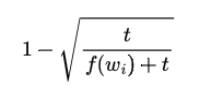
This is slightly different than the formula proposed by Mikolov et al., but it achieves a similar goal. The small difference is the +t component in the denominator. If the +t is excluded from the denominator, words with a frequency greater than t would be effectively removed from the data since the value in the square root would be greater than 1. This is the formula that is implemented in the _create_discard_dict() method, which creates a python dictionary where the key is a word index and the value is the probability of discarding it. The next question is where does t come from? Recall our Word2VecParams has the parameter T. This parameter is set to 85 in our code. This means that we find the 85th percentile word frequency and then set t to that value. This effectively makes the probability of randomly sampling a word with a frequency in the 85th percentile or above close to but slightly greater than 0%. This computation is what the _t() method in the SkipGram class achieves.
Creating our Negative Sampling Array
The final step before we define the PyTorch model is to create the negative sampling array. The high-level goal is to create an array of length 5,000,000 and populate it with vocabulary indices proportional to the frequency of the words in the vocabulary.
https://medium.com/media/04aa5f518c25fb47292643f79ffb65fd/hrefThe _create_negative_sampling() method creates the array exactly as specified above. The only slight difference is if a word has a frequency that implies it should have fewer than 1 entry in the negative sampling vector, we ensure that this word index is still present in 1 element of the negative sampling array so we don’t completely lose this word when we sample negative context words.
The sample() method returns a list of lists where the number of lists contained in the outer list is equal to the number of examples in the batch, and the number of samples within the inner lists is the number of negative samples for each example, which we have set to 50 in the Word2VecParams dataclass.
Defining the PyTorch Model
Finally, we get to build the word2vec model in PyTorch. The idiomatic approach to building a PyTorch neural network is to define the various network architecture layers in the constructor, and the forward pass of data through the network in a method called forward(). Luckily, PyTorch has abstracted away the backwards pass that updates the model parameters so we do not need to compute gradients manually.
https://medium.com/media/f97b3f639d6c699c0b44998f4aa34bee/hrefPyTorch models are always inherited from torch.nn.Module class. We will leverage the PyTorch embedding layer, which creates a lookup table of word vectors. The two layers we define in our word2vec model are self.t_embeddings, which is the target embeddings that we are interested in learning, and self.c_embeddings, which is the secondary (purple) embedding matrix from Figure 2. Both of these embedding matrices are initialized randomly.
If we wanted to train every parameter in the network, we could forego negative sampling at this point and the forward method would be a bit simpler. But, negative sampling has been shown to improve model accuracy and reduce training time so it is worth implementing. Let’s dig into the forward pass.
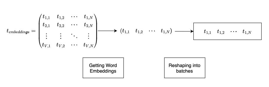
https://medium.com/media/5d1f504bdb578fda001019b2ca4e5bce/hrefLet’s imagine we have one training example we are passing through as a batch. In this example, inputs contains only the word associated with index 1. The first step of the forward pass is to lookup this word’s embeddings in the self.t_embeddings table. Then we use the .view() method to reshape it so we have an individual vector for the input we pass through the network. In the actual implementation, the batch size is 100. The .view() method creates a (1 x N)matrix for each word in each of the 100 training examples in the batch. Figure 4 will help the reader visualize what these first four lines of the forward() method do.
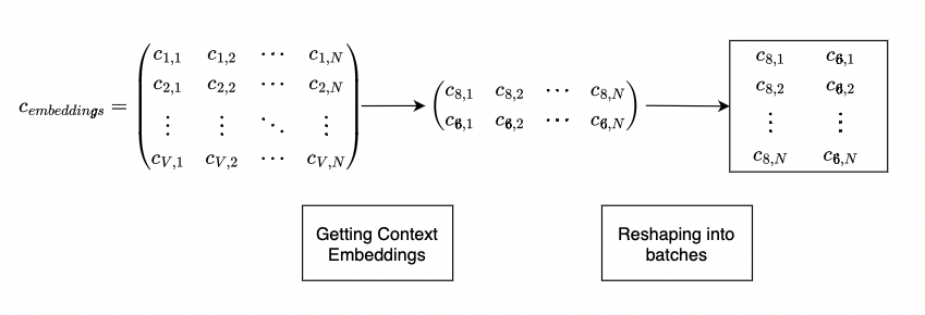
Then, for each of the inputs, we need to get the context word embeddings. For this example, say the actual context word is associated with the 8th index of the self.c_embeddings table and the negative context word is associated with the 6th index of the self.c_embeddings table. In this toy example, we are only using 1 negative sample. Figure 5 is a visualization of what these next two lines of PyTorch do.
The target embedding vector is of dimension (1 x N) and our context embedding matrix is of dimension (N x 2). So, our matrix multiplication results in a matrix of dimension (1 x 2). Figure 6 is what the final two lines of the forward() method accomplishes.
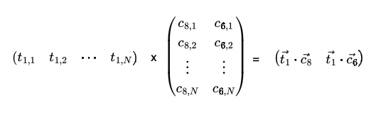
An alternative way to conceptualize this forward pass with negative sampling is by thinking of it as a dot product between the target word and each word in the context — the positive context word and all the negative context words. In this example, our positive context word was the 8th word in the vocabulary and the negative context word was the 6th word in the vocabulary. The resulting (1 x 2) vector contains the logits for the two context words. Since we know the first context word is the positive context word and the second context word is the negative context word, the value should be large for the first element and small for the second element. To achieve this, we will use the torch.nn.BCEWithLogitsLoss as the loss function. We will revisit the choice of loss function in a later section.
The last 3 methods in the Model class are normalize_embeddings(), get_similar_words(), and get_similarity(). Without getting into the details of each method, the normalize_embeddings() method scales every word embedding such that it is a unit vector (i.e., has a norm of 1). The get_similar_words() method will take a word and will return a list of the top-n most similar words. The similarity metric used is the cosine similarity. In other words, this method will return words whose vector representations are “closest” to the word of interest as measured by the angle between the two vectors. Finally, get_similarity() will take two words and will return the cosine similarity between the two word vectors.
Creating the Trainer
The final step of the process is to create a class that I called Trainer. The Trainer class code is as follows:
https://medium.com/media/1f84cb0a8c360c59ca7da3eb90363caa/hrefThis class will orchestrate all the previously developed code to train the model. The methods in this class are train(), _train_epoch(), _validate_epoch(), and test_testwords(). The train() method is the method we will call to start the model training. It loops over all the epochs and calls the _train_epoch() and validate_epoch() methods. After the epoch trains and is validated, it will print out the test words by calling the test_testwords() method so we can visually inspect if the embeddings are improving. The most critical methods in this class are the _train_epoch() and _validate_epoch() methods. These methods are very similar in what they do but have one small difference. Let’s dig into the _train_epoch() method.
https://medium.com/media/77ebdecf9d9ecda88d21d68b734f9ace/hrefWe first tell the model that it is in training mode usingself.model.train(). This allows PyTorch to make certain types of network layers behave as expected during training. These layer types are not implemented in this model, but it is a best practice to inform PyTorch that the model is training. The next step is to loop over each batch, get the positive and negative context words, and send them to the appropriate device (CPU or GPU). In other words, we create the context tensor, which accesses the batched data from the dataloaders we constructed with the SkipGrams class and concatenates it with negative samples we generated with our NegativeSampler class. Next we construct the ground truth tensor, y. Since we know the first element in the context tensor is the positive context word and all the following elements are the negative context words, we create a tensor, y, where the first element of the tensor is a 1 and all the following elements are 0s.
Now that we have our input data, the context data, and the ground truth labels, we can execute the forward pass. The first step is to tell PyTorch to set all the gradients to 0. Otherwise, each time we pass a batch of data through the model the gradient will be added, which is not the desired behavior. Then we execute the forward pass with the following line:
outputs = self.model(inputs, context)
Next, the loss is computed. We are using the torch.nn.BCEWithLogitsLoss objective function since we have a binary classification problem where the first element of the tensor, y, is 1 and the following elements are 0. For more information of this loss function, please refer to the documentation. Sebastian Raschka’s blog has a very good overview of binary cross entropy loss in PyTorch that can provide further insight, as well.
loss = self.params.CRITERION(outputs, y)
PyTorch will automatically compute the gradient during this loss computation. The gradient contains all the information needed to make small adjustments to the model parameters and decrease the loss. This automatic computation is done in the line:
loss.backward()
The small updates to the model parameters are done in the following line. Note, we are using the torch.optim.Adam optimizer . Adam is one of the most cutting edge convex optimization algorithms that is an descendant of stochastic gradient descent. I will not go into details about Adam in this post, but note that it tends to be one of the faster optimization algorithms since it leverages adaptive learning and gradient descent.
self.optimizer.step()
The _validate_epoch() method is identical to the _train_epoch() method except it does not keep track of the gradients nor does it update the model parameters with the optimizer step. This is all accomplished with the line with torch.no_grad(). Additionally, the _validate_epoch() method only uses the validation data, not the training data.
Putting it All Together
Below is the word2vec notebook in its entirety:
https://medium.com/media/dfb71fd03ea8aff74485acdceb7d0047/hrefI ran this notebook in Google Colab instance with a GPU. As you can see, I trained the model for 5 epochs with each epoch taking between 42 and 43 minutes. So, the whole notebook ran in under 4 hours. Please feel free to play around with it and provide any feedback or questions!
Results
https://medium.com/media/9fa0c36f95d31ed4587ffbb42b480e5a/hrefAfter training for just under 4 hours, observe the results in the snippet above. In addition to the decreasing loss, observe how the most similar words improved as the epochs trained. After the first epoch of training, the top 5 most similar words to military were: by, for, although, was, and any. After 5 epochs of training, the top 5 most similar words to military were: army, forces, officers, leadership, and soldiers. This, along with the decreasing loss, shows that the embeddings the model is learning are accurately representing the semantic meaning of the words in the vocabulary.
Thank you for reading! Please leave a comment if you found this helpful or you have any questions or concerns.
Conclusion
To conclude, we have reviewed a PyTorch implementation of word2vec with negative sampling and subsampling. This model allows us transform words into continuous vectors in an n-dimensional vector space. These embedding vectors are learned such that words with similar semantic meaning are grouped close together. With enough training data and sufficient time to train, the word2vec model can also learn syntactic patterns in text data. Word embeddings are a foundational component of NLP and are critical in more advanced models such as Transformer-based large language models. Having a thorough understanding of word2vec is an extremely helpful foundation for further NLP learning!
All images unless otherwise noted are by the author.
References
[1] T. Mikolov, K. Chen, G. Corrado, and J. Dean, Efficient Estimation of Word Representations in Vector Space (2013), Google Inc.
[2] T. Mikolov, I. Sutskever, K. Chen, G. Corrado, and J. Dean, Distributed Representations of Words and Phrases and their Compositionality (2013), Google Inc.
[3] S. Raschka, Losses Learned (2022), https://sebastianraschka.com
Implementing Word2vec in PyTorch from the Ground Up was originally published in Towards Data Science on Medium, where people are continuing the conversation by highlighting and responding to this story.
...