

 800+ IT
News
als RSS Feed abonnieren
800+ IT
News
als RSS Feed abonnieren📚 Reinforcement Learning for Inventory Optimization Series II: An RL Model for A Multi-Echelon…
💡 Newskategorie: AI Nachrichten
🔗 Quelle: towardsdatascience.com
Reinforcement Learning for Inventory Optimization Series II: An RL Model for A Multi-Echelon Network
Build a proximal policy optimization (PPO) model to optimize the inventory operations of a multi-echelon supply chain network

Update: this article is the second article in my blog series Reinforcement Learning for Inventory Optimization. Below is the link to the other article in the same series. Please check it out if you are interested.
Reinforcement Learning for Inventory Optimization Series I: An RL Model for Single Retailers
In my previous article, I presented a DQN model for optimizing the inventory control policy of a single retailer whose customer demand pattern can be described by a mixture of normal distributions. The DQN model achieved significantly better results as compared to a traditional (s, S) inventory control policy. In this article, as mentioned at the end of my previous article, I’m going to take one step further in RL for inventory optimization and focus on building an RL model for more complex supply chain networks — multi-echelon networks.
Challenges in RL Modeling for A Multi-Echelon Network
Undoubtedly, building an RL model for a multi-echelon network is far more complicated than for a single retailer. The complication comes from the fact that the increase of entities in the supply chain causes scalability issues. In the single retailer example in the previous article, we are only concerned with the inventory control policy for one entity — the retailer. Hence, it suffices to build only one agent with an action space denoting the order quantity of the retailer. However, a multi-echelon network is a more complex system usually involving entities of different types (e.g., manufacturing plant, distribution center, retailer, etc.).
To model such a system, we have two possible approaches. The first approach would be to model each entity as an independent agent and build a multi-agent RL model. In this approach, each agent cares about the action of only one entity in the network, which fairly limits the the size of the action space. However, multi-agent RL models are often much harder to train and tune as compared to single-agent RL models, since the success of the entire model depends on the good training and tuning of every agent, and also on the cooperations between agents. The second approach would be to model the whole network using a single agent, with an action space flexible enough to describe the ordering decisions of all entities simultaneously, e.g., an n-dimensional action space with each dimension corresponding to the ordering decision of each entity. However, the drawback of this approach is the dramatic increase of the size of action space as the number of entities scales up. The size of the action space increases exponentially with the number of entities.
An RL Model for A Simple Multi-Echelon Network
Let’s resume from the example in the previous article. Assume that there is a retail company with retail stores opened in different regions across the country selling Coke for profit. Instead of focusing on the inventory operations of one single retail store in the previous article, here we assume the retail company has its own distribution centers (DCs) to fulfill the demands of its retail stores, and we seek to optimize the inventory control policy of an entire network consisting of DCs and retail stores.
To make the example simpler, we consider a multi-echelon network consisting of only two distribution centers (DCs) and four retailers. The transportation links between DCs and retailers are depicted by the figure below.
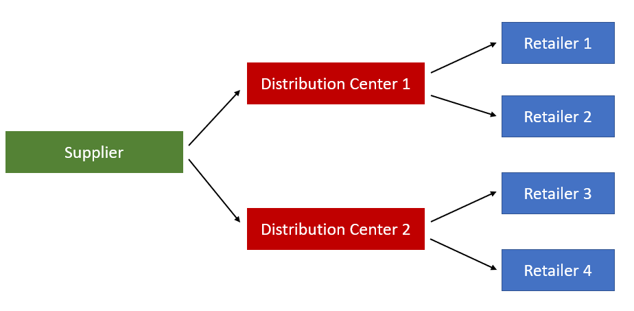
We see that the retail company first buys Coke from its supplier, then transport the Coke to DC 1 and DC 2. DC 1 stores inventory to fulfill the orders from retailer 1 and retailer 2, and DC 2 stores inventory to fulfill the orders from retailer 3 and retailer 4. In this example, let’s further assume that all the four retailers have the same customer demand pattern as in the previous article. Specifically, the customer demands at all four retailers follow a mixture of normal distributions, where the demand from Monday to Thursday follows a normal distribution with the lowest mean, the demand on Friday follows a normal distribution with the medium mean, and the demand from Saturday to Sunday follows a normal distribution with the highest mean.
For this particular problem, one thing to notice is that the whole network can be decomposed into two sub-networks with one consisting DC 1, retailer 1 and retailer 2, and the other consisting of DC 2, retailer 3 and retailer 4. These two sub-networks have the same customer demand distribution. Hence, to make the training process easier, we can adopt a divide and conquer methodology here. Instead of modeling the whole network, we only model the sub-network by one RL agent, and we train the RL agent using the data from the first and second sub-network sequentially. The state, action, and reward definitions of the RL model are given as follows:
- State: (i_pt_dc1, i_pt_r1, i_pt_r2, dow_t), where i_pt_dc1 is the inventory position of DC 1 at the end of tth day, i_pt_r1 is the inventory position of retailer 1, i_pt_r2 is the inventory position of retailer 2, and and dow_t is a 6-dimensional vector representation of the day of week of the tth day using one hot encoding.
- Action: (a_t_dc1, a_t_r1, a_t_r2), where a_t_dc1 is the order quantity of DC 1 at the end of tth day, a_t_r1 is the order quantity of retailer 1 at the end of tth day, and a_t_r2 is the order quantity of retailer 2 at the end of tth day. Note that if a_t_dc1, a_t_r1 or a_t_r2 is 0, then we don’t place an order for the corresponding entity at that time. The action space is limited by the maximum order quantity, determined by suppliers or the capacity of transportation vehicles.
- Reward: r_t = r_t_r1+r_t_r2-h_t_r1-h_t_r2-h_t_dc1-f_t_r1-f_t_r2-f_t_dc1-v_t_dc1, where r_t_r1 and r_t_r2 are the revenues obtained by selling the product at retailer 1 and 2 during the daytime of (t+1)th day, h_t_r1, h_t_r2 and h_t_dc1 are the holding costs incurred at retailer 1, 2 and DC 1 at the tth night, f_t_r1, f_t_r2 and f_t_dc1 are the fixed ordering costs (e.g., delivery fee) incurred at retailer 1, 2 and DC 1 during the tth decision epoch, and v_t_dc1 is the variable ordering cost (purchase cost of the product charged by the supplier) incurred at DC 1 at the end of tth day. Since we assume the variable ordering cost only refers to the purchase cost, we only need to calculate this cost at DC 1. It’s easy to see that the reward r_t is just the profit obtained in the tth decision epoch from the sub-network consisting of DC 1, retailer 1 and retailer 2.
Note that this modeling framework follows the second modeling approach mentioned in the previous section, and it may suffer from the curse of dimensionality. If we assume the action for each entity to take discrete values from 0 to a_max (the maximum order quantity), then the size of the action space increases exponentially with the number of entities in the network. This causes difficulties for effectively training the RL agent. One way to mitigate this issue is to restrict the the values that an action can take within the [0, a_max] interval. For example, if a_max = 20, we can impose a restriction that the action can only take values 0, 5, 15 or 20, instead of allowing it to take every single integer between 0 and 20. This may somewhat undermine the optimality of the resulting policy obtained from the RL agent, but it can significantly reduce the size of the action space.
Numerical Experiment
Assume there is a small retail company which sells Coke to its customers. The retail company has two DCs and four retailers to fulfill customer demand. Every time the company wants to replenish its inventory at any DC or retailer, the company has to place an order of an integer number of cases of Coke (one case contains 24 cans). Suppose that for retailers, the unit selling price of Coke is $30 per case, holding cost is $3 per case per night, fixed ordering cost is $50 per order, the inventory capacity is 50 cases, the maximum order quantity allowed is 20 cases per order, the initial inventory is 25 cases at the end of a Sunday, and the lead time is 2 days. The demand from Monday to Thursday follows a normal distribution N(3,1.5), the demand on Friday follows a normal distribution N(6,1), and the demand from Saturday to Sunday follows a normal distribution N(12,2). For DCs, the holding cost is $1 per case per night, fixed ordering cost is $75 per order, the inventory capacity is 200 cases, the maximum order quantity allowed is 100 cases per order, the initial inventory is 100 cases at the end of a Sunday, and the lead time is 5 days. We generate 52 weeks of historical demand samples from the mixture of distributions, and use this as a training dataset for the RL model.
Regarding the choice of the specific RL algorithm to use, I adopted the proximal policy optimization (PPO) algorithm as it is a state-of-the-art policy-based RL algorithm which is able to give a stochastic policy. I also tried using value-based algorithms producing a deterministic policy (e.g., DQN), but found PPO to be more effective for this particular example. Here, I omit the detailed explanation of the PPO algorithm as it is not the focus of this article. Interested readers are referred to this article for more details.
As a benchmark, we will optimize a classic (s,S) inventory control policy using the same dataset which was used for training the PPO model, and compare its performance with PPO in a test set.
Code for training the PPO model
First, we generate the training dataset which contains 52 weeks of historical demand records of the four retailers. Note that non-integer demand data are rounded to nearest integers.
import numpy as np
import matplotlib.pyplot as plt
import random
np.random.seed(0)
demand_hist_list = []
for k in range(4):
    demand_hist = []
    for i in range(52):
        for j in range(4):
            random_demand = np.random.normal(3, 1.5)
            if random_demand < 0:
                random_demand = 0
            random_demand = np.round(random_demand)
            demand_hist.append(random_demand)
        random_demand = np.random.normal(6, 1)
        if random_demand < 0:
            random_demand = 0
        random_demand = np.round(random_demand)
        demand_hist.append(random_demand)
        for j in range(2):
            random_demand = np.random.normal(12, 2)
            if random_demand < 0:
                random_demand = 0
            random_demand = np.round(random_demand)
            demand_hist.append(random_demand)
    demand_hist_list.append(demand_hist)
Then we define the environment of the inventory optimization problem for the PPO agent to interact with. The environment contains a sub-network with one DC and two retailers. In this example, backorders are not considered for retailers, as we assume if customers don’t see any Coke left in the retailer stores, they will go to other stores to buy Coke. However, backorders are considered for the DC. When the DC does not have enough inventory to fulfill the orders of the retailers, a backorder occurs, and the DC will fulfill the backorder as soon as it replenishes the inventory. To restrict the size of the action space, we allow the order quantity of the DC to take values in [0, 10, 20, 30, 40, 50, 60, 70, 80, 90, 100], and the two retailers to take values in [0, 5, 10, 15, 20]. The size of the action space is now 11*5*5 = 275.
import itertools
action_lists = [[0, 10, 20, 30, 40, 50, 60, 70, 80, 90, 100],[0, 5, 10, 15, 20],[0, 5, 10, 15, 20]]
action_map = [x for x in itertools.product(*action_lists)]

class Retailer():
    def __init__(self, demand_records):
        self.inv_level = 25
        self.inv_pos = 25
        self.order_quantity_limit = 20
        self.holding_cost = 3
        self.lead_time = 2
        self.order_arrival_list = []
        self.backorder_quantity = 0
        self.capacity = 50
        self.demand_list = demand_records
        self.unit_price = 30
        self.fixed_order_cost = 50

    def reset(self):
        self.inv_level = 25
        self.inv_pos = 25
        self.order_arrival_list = []
        self.backorder_quantity = 0

    def order_arrival(self, current_period):
        n_orders = 0
        if len(self.order_arrival_list) > 0:
            index_list = []
            for j in range(len(self.order_arrival_list)):
                if current_period == self.order_arrival_list[j][0]:
                    self.inv_level = min(self.capacity, self.inv_level + self.order_arrival_list[j][1])
                    n_orders += 1
                    index_list.append(j)
            self.order_arrival_list =  [e for i, e in enumerate(self.order_arrival_list) if i not in index_list]
        holding_cost_total = self.inv_level*self.holding_cost
        return n_orders, holding_cost_total

    def satisfy_demand(self, demand):
        units_sold = min(demand, self.inv_level)
        self.inv_level = max(0,self.inv_level-demand)
        self.inv_pos = self.inv_level
        if len(self.order_arrival_list) > 0:
            for j in range(len(self.order_arrival_list)):
                self.inv_pos += self.order_arrival_list[j][1]
        revenue = units_sold*self.unit_price
        return revenue

class DistributionCenter():
    def __init__(self):
        self.inv_level = 100
        self.inv_pos = 100
        self.order_quantity_limit = 100
        self.holding_cost = 1
        self.lead_time = 5
        self.order_arrival_list = []
        self.capacity = 200
        self.fixed_order_cost = 75

    def reset(self):
        self.inv_level = 100
        self.inv_pos = 100
        self.order_arrival_list = []

    def place_order(self, order_quantity, current_period):
        if order_quantity > 0:
            self.order_arrival_list.append([current_period+self.lead_time, order_quantity])

    def order_arrival(self, retailers, current_period):
        if len(self.order_arrival_list) > 0:
            if current_period == self.order_arrival_list[0][0]:
                self.inv_level = min(self.capacity, self.inv_level+self.order_arrival_list[0][1])
                self.order_arrival_list.pop(0)
        holding_cost_total = self.inv_level*self.holding_cost
        return holding_cost_total

    def satisfy_demand(self, retailers, actions, current_period):
        quantity_satisfied = [0,0]
        total_backorder = np.sum([retailer.backorder_quantity for retailer in retailers])
        if total_backorder > 0:
            if self.inv_level <= retailers[0].backorder_quantity:
                retailers[0].backorder_quantity -= self.inv_level
                quantity_satisfied[0] += self.inv_level
                self.inv_level = 0
            if self.inv_level > retailers[0].backorder_quantity and self.inv_level <= total_backorder:
                if retailers[0].backorder_quantity == 0:
                    retailers[1].backorder_quantity -= self.inv_level
                    quantity_satisfied[1] += self.inv_level
                else:
                    quantity_left = self.inv_level - retailers[0].backorder_quantity
                    quantity_satisfied[0] += retailers[0].backorder_quantity
                    retailers[0].backorder_quantity = 0
                    quantity_satisfied[1] += quantity_left
                    retailers[1].backorder_quantity -= quantity_left
                self.inv_level = 0
            if self.inv_level > total_backorder:
                if retailers[0].backorder_quantity == 0 and retailers[1].backorder_quantity != 0:
                    quantity_satisfied[1] += retailers[1].backorder_quantity
                    retailers[1].backorder_quantity = 0
                if retailers[0].backorder_quantity != 0 and retailers[1].backorder_quantity == 0:
                    quantity_satisfied[0] += retailers[0].backorder_quantity
                    retailers[0].backorder_quantity = 0
                if retailers[0].backorder_quantity != 0 and retailers[1].backorder_quantity != 0:
                    quantity_satisfied[0] += retailers[0].backorder_quantity
                    quantity_satisfied[1] += retailers[1].backorder_quantity
                    retailers[0].backorder_quantity = 0
                    retailers[1].backorder_quantity = 0
                self.inv_level -= total_backorder

        if self.inv_level > 0:
            if self.inv_level <= actions[0]:
                quantity_satisfied[0] += self.inv_level
                retailers[0].backorder_quantity += actions[0] - self.inv_level
                self.inv_level = 0
            if self.inv_level > actions[0] and self.inv_level <= np.sum(actions):
                if actions[0] == 0:
                    quantity_satisfied[1] += self.inv_level
                    retailers[1].backorder_quantity += actions[1] - self.inv_level
                else:
                    inv_left = self.inv_level-actions[0]
                    quantity_satisfied[0] += actions[0]
                    quantity_satisfied[1] += inv_left
                    retailers[1].backorder_quantity += actions[1] - inv_left
                self.inv_level = 0
            if self.inv_level > np.sum(actions):
                if actions[0] == 0 and actions[1] != 0:
                    quantity_satisfied[1] += actions[1]
                if actions[0] != 0 and actions[1] == 0:
                    quantity_satisfied[0] += actions[0]
                if actions[0] != 0 and actions[1] != 0:
                    quantity_satisfied[0] += actions[0]
                    quantity_satisfied[1] += actions[1]
                self.inv_level -= np.sum(actions)
        else:
            retailers[0].backorder_quantity += actions[0]
            retailers[1].backorder_quantity += actions[1]

        for i in range(len(retailers)):
            quantity_left = quantity_satisfied[i]
            while quantity_left > 0:
                if quantity_left > retailers[i].order_quantity_limit:
                    retailers[i].order_arrival_list.append([current_period+retailers[i].lead_time, retailers[i].order_quantity_limit])
                    quantity_left -= retailers[i].order_quantity_limit
                else:
                    retailers[i].order_arrival_list.append([current_period+retailers[i].lead_time, quantity_left])
                    quantity_left = 0

        self.inv_pos = self.inv_level
        if len(self.order_arrival_list) > 0:
            for j in range(len(self.order_arrival_list)):
                self.inv_pos += self.order_arrival_list[j][1]
        for retailer in retailers:
            self.inv_pos -= retailer.backorder_quantity


class MultiEchelonInvOptEnv():
    def __init__(self, demand_records):
        self.n_retailers = 2
        self.n_DCs = 1
        self.retailers = []
        for i in range(self.n_retailers):
            self.retailers.append(Retailer(demand_records[i]))
        self.DCs = []
        for i in range(self.n_DCs):
            self.DCs.append(DistributionCenter())
        self.n_period = len(demand_records[0])
        self.current_period = 1
        self.day_of_week = 0
        self.state = np.array([DC.inv_pos for DC in self.DCs] + [retailer.inv_pos for retailer in self.retailers] + \
                              self.convert_day_of_week(self.day_of_week))
        self.variable_order_cost = 10
        self.demand_records = demand_records

    def reset(self):
        for retailer in self.retailers:
            retailer.reset()
        for DC in self.DCs:
            DC.reset()
        self.current_period = 1
        self.day_of_week = 0
        self.state = np.array([DC.inv_pos for DC in self.DCs] + [retailer.inv_pos for retailer in self.retailers] + \
                              self.convert_day_of_week(self.day_of_week))
        return self.state

    def step(self, action):
        action_modified = action_map[action]
        y_list = []
        for i in range(self.n_DCs):
            y = 1 if action_modified[i] > 0 else 0
            y_list.append(y)
        for DC,order_quantity in zip(self.DCs,action_modified[:self.n_DCs]):
            DC.place_order(order_quantity,self.current_period)
        sum_holding_cost_DC = 0
        for i in range(self.n_DCs):
            holding_cost_total = self.DCs[i].order_arrival(self.retailers,self.current_period)
            sum_holding_cost_DC += holding_cost_total
            self.DCs[i].satisfy_demand(self.retailers,action_modified[i*2+1:i*2+3],self.current_period)
        sum_n_orders = 0
        sum_holding_cost_retailer = 0
        sum_revenue = 0
        for retailer,demand in zip(self.retailers,self.demand_records):
            n_orders, holding_cost_total = retailer.order_arrival(self.current_period)
            sum_n_orders += n_orders
            sum_holding_cost_retailer += holding_cost_total
            revenue = retailer.satisfy_demand(demand[self.current_period-1])
            sum_revenue += revenue
        reward = sum_revenue - sum_holding_cost_retailer - sum_holding_cost_DC - sum_n_orders*self.retailers[0].fixed_order_cost - \
                 np.sum(y_list)*self.DCs[0].fixed_order_cost - np.sum(action_modified[:self.n_DCs])*self.variable_order_cost

        self.day_of_week = (self.day_of_week+1)%7
        self.state = np.array([DC.inv_pos for DC in self.DCs] + [retailer.inv_pos for retailer in self.retailers] + \
                              self.convert_day_of_week(self.day_of_week))
        self.current_period += 1
        if self.current_period > self.n_period:
            terminate = True
        else:
            terminate = False
        return self.state, reward, terminate

    def convert_day_of_week(self,d):
        if d == 0:
            return [0, 0, 0, 0, 0, 0]
        if d == 1:
            return [1, 0, 0, 0, 0, 0]
        if d == 2:
            return [0, 1, 0, 0, 0, 0]
        if d == 3:
            return [0, 0, 1, 0, 0, 0]
        if d == 4:
            return [0, 0, 0, 1, 0, 0]
        if d == 5:
            return [0, 0, 0, 0, 1, 0]
        if d == 6:
            return [0, 0, 0, 0, 0, 1]
Now we begin building the PPO model with PyTorch. The implementation of PPO in this part is based on this repository.
import torch
import torch.nn as nn
from torch.distributions import MultivariateNormal
from torch.distributions import Categorical

################################## set device ##################################
print("============================================================================================")
# set device to cpu or cuda
device = torch.device('cpu')
if(torch.cuda.is_available()):
    device = torch.device('cuda:0')
    torch.cuda.empty_cache()
    print("Device set to : " + str(torch.cuda.get_device_name(device)))
else:
    print("Device set to : cpu")
print("============================================================================================")


################################## PPO Policy ##################################
class RolloutBuffer:
    def __init__(self):
        self.actions = []
        self.states = []
        self.logprobs = []
        self.rewards = []
        self.is_terminals = []

    def clear(self):
        del self.actions[:]
        del self.states[:]
        del self.logprobs[:]
        del self.rewards[:]
        del self.is_terminals[:]


class ActorCritic(nn.Module):
    def __init__(self, state_dim, action_dim, has_continuous_action_space, action_std_init):
        super(ActorCritic, self).__init__()

        self.has_continuous_action_space = has_continuous_action_space

        if has_continuous_action_space:
            self.action_dim = action_dim
            self.action_var = torch.full((action_dim,), action_std_init * action_std_init).to(device)
        # actor
        if has_continuous_action_space :
            self.actor = nn.Sequential(
                            nn.Linear(state_dim, 256),
                            nn.Tanh(),
                            nn.Linear(256,256),
                            nn.Tanh(),
                            nn.Linear(256, action_dim),
                            nn.Sigmoid()
                        )
        else:
            self.actor = nn.Sequential(
                            nn.Linear(state_dim, 384),
                            nn.Tanh(),
                            nn.Linear(384, 384),
                            nn.Tanh(),
                            nn.Linear(384, action_dim),
                            nn.Softmax(dim=-1)
                        )
        # critic
        self.critic = nn.Sequential(
                        nn.Linear(state_dim, 128),
                        nn.Tanh(),
                        nn.Linear(128, 128),
                        nn.Tanh(),
                        nn.Linear(128, 1)
                    )

    def set_action_std(self, new_action_std):
        if self.has_continuous_action_space:
            self.action_var = torch.full((self.action_dim,), new_action_std * new_action_std).to(device)
        else:
            print("--------------------------------------------------------------------------------------------")
            print("WARNING : Calling ActorCritic::set_action_std() on discrete action space policy")
            print("--------------------------------------------------------------------------------------------")

    def forward(self):
        raise NotImplementedError

    def act(self, state):
        if self.has_continuous_action_space:
            action_mean = self.actor(state)
            cov_mat = torch.diag(self.action_var).unsqueeze(dim=0)
            dist = MultivariateNormal(action_mean, cov_mat)
        else:
            action_probs = self.actor(state)
            dist = Categorical(action_probs)

        action = dist.sample()
        action_logprob = dist.log_prob(action)

        return action.detach(), action_logprob.detach()

    def evaluate(self, state, action):

        if self.has_continuous_action_space:
            action_mean = self.actor(state)

            action_var = self.action_var.expand_as(action_mean)
            cov_mat = torch.diag_embed(action_var).to(device)
            dist = MultivariateNormal(action_mean, cov_mat)

            # For Single Action Environments.
            if self.action_dim == 1:
                action = action.reshape(-1, self.action_dim)
        else:
            action_probs = self.actor(state)
            dist = Categorical(action_probs)
        action_logprobs = dist.log_prob(action)
        dist_entropy = dist.entropy()
        state_values = self.critic(state)

        return action_logprobs, state_values, dist_entropy


class PPO:
    def __init__(self, state_dim, action_dim, lr_actor, lr_critic, gamma, K_epochs, eps_clip, has_continuous_action_space, action_std_init=0.6):

        self.has_continuous_action_space = has_continuous_action_space

        if has_continuous_action_space:
            self.action_std = action_std_init

        self.gamma = gamma
        self.eps_clip = eps_clip
        self.K_epochs = K_epochs

        self.buffer = RolloutBuffer()

        self.policy = ActorCritic(state_dim, action_dim, has_continuous_action_space, action_std_init).to(device)
        self.optimizer = torch.optim.Adam([
                        {'params': self.policy.actor.parameters(), 'lr': lr_actor},
                        {'params': self.policy.critic.parameters(), 'lr': lr_critic}
                    ])

        self.policy_old = ActorCritic(state_dim, action_dim, has_continuous_action_space, action_std_init).to(device)
        self.policy_old.load_state_dict(self.policy.state_dict())

        self.MseLoss = nn.MSELoss()

    def set_action_std(self, new_action_std):
        if self.has_continuous_action_space:
            self.action_std = new_action_std
            self.policy.set_action_std(new_action_std)
            self.policy_old.set_action_std(new_action_std)
        else:
            print("--------------------------------------------------------------------------------------------")
            print("WARNING : Calling PPO::set_action_std() on discrete action space policy")
            print("--------------------------------------------------------------------------------------------")

    def decay_action_std(self, action_std_decay_rate, min_action_std):
        print("--------------------------------------------------------------------------------------------")
        if self.has_continuous_action_space:
            self.action_std = self.action_std - action_std_decay_rate
            self.action_std = round(self.action_std, 4)
            if (self.action_std <= min_action_std):
                self.action_std = min_action_std
                print("setting actor output action_std to min_action_std : ", self.action_std)
            else:
                print("setting actor output action_std to : ", self.action_std)
            self.set_action_std(self.action_std)

        else:
            print("WARNING : Calling PPO::decay_action_std() on discrete action space policy")
        print("--------------------------------------------------------------------------------------------")

    def select_action(self, state):

        if self.has_continuous_action_space:
            with torch.no_grad():
                state = torch.FloatTensor(state).to(device)
                action, action_logprob = self.policy_old.act(state)

            self.buffer.states.append(state)
            self.buffer.actions.append(action)
            self.buffer.logprobs.append(action_logprob)

            return action.detach().cpu().numpy().flatten()
        else:
            with torch.no_grad():
                state = torch.FloatTensor(state).to(device)
                action, action_logprob = self.policy_old.act(state)

            self.buffer.states.append(state)
            self.buffer.actions.append(action)
            self.buffer.logprobs.append(action_logprob)

            return action.item()

    def update(self):
        # Monte Carlo estimate of returns
        rewards = []
        discounted_reward = 0
        for reward, is_terminal in zip(reversed(self.buffer.rewards), reversed(self.buffer.is_terminals)):
            if is_terminal:
                discounted_reward = 0
            discounted_reward = reward + (self.gamma * discounted_reward)
            rewards.insert(0, discounted_reward)

        # Normalizing the rewards
        rewards = torch.tensor(rewards, dtype=torch.float32).to(device)
        rewards = (rewards - rewards.mean()) / (rewards.std() + 1e-7)

        # convert list to tensor
        old_states = torch.squeeze(torch.stack(self.buffer.states, dim=0)).detach().to(device)
        old_actions = torch.squeeze(torch.stack(self.buffer.actions, dim=0)).detach().to(device)
        old_logprobs = torch.squeeze(torch.stack(self.buffer.logprobs, dim=0)).detach().to(device)

        # Optimize policy for K epochs
        for _ in range(self.K_epochs):

            # Evaluating old actions and values
            logprobs, state_values, dist_entropy = self.policy.evaluate(old_states, old_actions)

            # match state_values tensor dimensions with rewards tensor
            state_values = torch.squeeze(state_values)

            # Finding the ratio (pi_theta / pi_theta__old)
            ratios = torch.exp(logprobs - old_logprobs.detach())

            # Finding Surrogate Loss
            advantages = rewards - state_values.detach()
            surr1 = ratios * advantages
            surr2 = torch.clamp(ratios, 1-self.eps_clip, 1+self.eps_clip) * advantages

            # final loss of clipped objective PPO
            loss = -torch.min(surr1, surr2) + 0.5*self.MseLoss(state_values, rewards) - 0.01*dist_entropy

            # take gradient step
            self.optimizer.zero_grad()
            loss.mean().backward()
            self.optimizer.step()

        # Copy new weights into old policy
        self.policy_old.load_state_dict(self.policy.state_dict())

        # clear buffer
        self.buffer.clear()
import os
import glob
import time
from datetime import datetime

import torch
import numpy as np

################################### Training ###################################
def train():
    print("============================================================================================")


    has_continuous_action_space = False # continuous action space; else discrete

    max_ep_len = 364                   # max timesteps in one episode
    max_training_timesteps = int(364*15000)   # break training loop if timeteps > max_training_timesteps

    print_freq = max_ep_len * 10        # print avg reward in the interval (in num timesteps)

    action_std = 0.6            # starting std for action distribution (Multivariate Normal)
    action_std_decay_rate = 0.03       # linearly decay action_std (action_std = action_std - action_std_decay_rate)
    min_action_std = 0.03               # minimum action_std (stop decay after action_std <= min_action_std)
    action_std_decay_freq = int(1e5)  # action_std decay frequency (in num timesteps)
    #####################################################

    ## Note : print/log frequencies should be > than max_ep_len

    ################ PPO hyperparameters ################
    update_timestep = max_ep_len/2       # update policy every n timesteps
    K_epochs = 20               # update policy for K epochs in one PPO update

    eps_clip = 0.2          # clip parameter for PPO
    gamma = 0.99            # discount factor

    lr_actor = 0.00005       # learning rate for actor network
    lr_critic = 0.0001       # learning rate for critic network

    random_seed = 0         # set random seed if required (0 = no random seed)
    #####################################################

    state_dim = 9
    action_dim = 275

    torch.manual_seed(random_seed)
    np.random.seed(random_seed)

    ################# training procedure ################

    # initialize a PPO agent
    ppo_agent = PPO(state_dim, action_dim, lr_actor, lr_critic, gamma, K_epochs, eps_clip, has_continuous_action_space, action_std)

    # track total training time
    start_time = datetime.now().replace(microsecond=0)
    print("Started training at (GMT) : ", start_time)

    print("============================================================================================")


    # printing and logging variables
    print_running_reward = 0
    print_running_episodes = 0

    time_step = 0
    i_episode = 0

    # training loop
    for i in range(2):
        env = MultiEchelonInvOptEnv(demand_hist_list[i*2:i*2+2])
        while time_step <= max_training_timesteps:

            state = env.reset()
            current_ep_reward = 0

            for t in range(1, max_ep_len+1):

                # select action with policy

                action = ppo_agent.select_action(state)
                state, reward, done = env.step(action)

                # saving reward and is_terminals
                ppo_agent.buffer.rewards.append(reward)
                ppo_agent.buffer.is_terminals.append(done)

                time_step +=1
                current_ep_reward += reward

                # update PPO agent
                if time_step % update_timestep == 0:
                    ppo_agent.update()

                # if continuous action space; then decay action std of ouput action distribution
                if has_continuous_action_space and time_step % action_std_decay_freq == 0:
                    ppo_agent.decay_action_std(action_std_decay_rate, min_action_std)


                # printing average reward
                if time_step % print_freq == 0:

                    # print average reward till last episode
                    print_avg_reward = print_running_reward / print_running_episodes
                    print_avg_reward = round(print_avg_reward, 2)

                    print("Episode : {} \t\t Timestep : {} \t\t Average Reward : {}".format(i_episode, time_step, print_avg_reward))

                    print_running_reward = 0
                    print_running_episodes = 0

                # break; if the episode is over
                if done:
                    break

            print_running_reward += current_ep_reward
            print_running_episodes += 1

            i_episode += 1
    torch.save(ppo_agent.policy.state_dict(), desired_path)

if __name__ == '__main__':

    train()
Code for optimizing the (s,S) policy
For this particular numerical experiment, the number of possible (s,S) combinations is prohibitively large. Hence, it’s impractical to enumerate all the possible combinations to optimize the (s,S) policy. Here, we adopt Bayesian optimization (BO) to obtain the optimal (s,S) policy. BO is a black-box optimization approach. It optimizes the objective function by sequentially sampling from the objective function and updating a surrogate model which approximates the objective function. BO uses an acquisition function to determine where to sample the next point, and the accuracy of the surrogate model gets improved continuously as more points are sampled. In the end, BO returns the point with the best objective function value among all the previously sampled points as the optimal solution. For more detailed introduction on BO, interested readers are referred to this article. The implementation of BO in this part is based on this repository.
In the code, we define an objective function with 6 parameters, namely s_DC, S_DC, s_r1, S_r1, s_r2, S_r2. The objective function calculates the profit obtained on the historical demand dataset, s_DC and S_DC define the (s,S) policy for two DCs, s_r1 and S_r1 define the (s,S) policy for retailer 1 and retailer 3, s_r2 and S_r2 define the (s,S) policy for retailer 2 and retailer 4. We then optimize this function using BO. We set the upper bound for S_DC to 210, giving a little extra room to allow S to take a value higher than the capacity. I tried setting the upper bound for S_r1 and S_r2 to each value from [60,70,80,90,100] and found that 90 gave the best objective value. Hence, I selected 90 as the upper bound. The best solution on the historical demand dataset turned out to be (s_DC, S_DC, s_r1, S_r1, s_r2, S_r2) = (62, 120, 15, 41, 17, 90).
def MultiEchelonInvOpt_sS(s_DC,S_DC,s_r1,S_r1,s_r2,S_r2):
    if s_DC > S_DC-1 or s_r1 > S_r1-1 or s_r2 > S_r2-1:
        return -1e8
    else:
        n_retailers = 4
        n_DCs = 2
        retailers = []
        for i in range(n_retailers):
            retailers.append(Retailer(demand_hist_list[i]))
        DCs = []
        for i in range(n_DCs):
            DCs.append(DistributionCenter())
        n_period = len(demand_hist_list[0])
        variable_order_cost = 10
        current_period = 1
        total_reward = 0
        while current_period <= n_period:
            action = []
            for DC in DCs:
                if DC.inv_pos <= s_DC:
                    action.append(np.round(min(DC.order_quantity_limit,S_DC-DC.inv_pos)))
                else:
                    action.append(0)
            for i in range(len(retailers)):
                if i%2 == 0:
                    if retailers[i].inv_pos <= s_r1:
                        action.append(np.round(min(retailers[i].order_quantity_limit,S_r1-retailers[i].inv_pos)))
                    else:
                        action.append(0)
                else:
                    if retailers[i].inv_pos <= s_r2:
                        action.append(np.round(min(retailers[i].order_quantity_limit,S_r2-retailers[i].inv_pos)))
                    else:
                        action.append(0)
            y_list = []
            for i in range(n_DCs):
                y = 1 if action[i] > 0 else 0
                y_list.append(y)
            for DC,order_quantity in zip(DCs,action[:n_DCs]):
                DC.place_order(order_quantity,current_period)
            sum_holding_cost_DC = 0
            for i in range(n_DCs):
                holding_cost_total = DCs[i].order_arrival(retailers[i*2:i*2+2],current_period)
                sum_holding_cost_DC += holding_cost_total
                DCs[i].satisfy_demand(retailers[i*2:i*2+2],action[i*2+2:i*2+4],current_period)
            sum_n_orders = 0
            sum_holding_cost_retailer = 0
            sum_revenue = 0
            for retailer,demand in zip(retailers,demand_hist_list):
                n_orders, holding_cost_total = retailer.order_arrival(current_period)
                sum_n_orders += n_orders
                sum_holding_cost_retailer += holding_cost_total
                revenue = retailer.satisfy_demand(demand[current_period-1])
                sum_revenue += revenue
            reward = sum_revenue - sum_holding_cost_retailer - sum_holding_cost_DC - sum_n_orders*retailers[0].fixed_order_cost - \
                     np.sum(y_list)*DCs[0].fixed_order_cost - np.sum(action[:n_DCs])*variable_order_cost

            current_period += 1
            total_reward += reward
        return total_reward
from bayes_opt import BayesianOptimization
pbounds = {'s_DC': (0,210), 'S_DC': (0, 210), 's_r1': (0, 90), 'S_r1': (0, 90), 's_r2': (0, 90), 'S_r2': (0, 90)}
optimizer = BayesianOptimization(
    f=MultiEchelonInvOpt_sS,
    pbounds=pbounds,
    random_state=0,
)
optimizer.maximize(
    init_points = 100,
    n_iter=1000
)
print(optimizer.max)
Code for testing the PPO policy
We first create 100 customer demand datasets for testing. Each of the 100 datasets contains 52 weeks of demand data for four retailers. We can think of each dataset as a possible scenario of the demands in the next 1 year. Then we evaluate the PPO policy on each demand dataset and collect the total reward for each dataset.
np.random.seed(0)
demand_test = []
for k in range(100,200):
    demand_list = []
    for k in range(4):
        demand = []
        for i in range(52):
            for j in range(4):
                random_demand = np.random.normal(3, 1.5)
                if random_demand < 0:
                    random_demand = 0
                random_demand = np.round(random_demand)
                demand.append(random_demand)
            random_demand = np.random.normal(6, 1)
            if random_demand < 0:
                random_demand = 0
            random_demand = np.round(random_demand)
            demand.append(random_demand)
            for j in range(2):
                random_demand = np.random.normal(12, 2)
                if random_demand < 0:
                    random_demand = 0
                random_demand = np.round(random_demand)
                demand.append(random_demand)
        demand_list.append(demand)
    demand_test.append(demand_list)
import os
import glob
import time
from datetime import datetime

import torch
import numpy as np

has_continuous_action_space = False # continuous action space; else discrete
action_std = 0.6            # starting std for action distribution (Multivariate Normal)
action_std_decay_rate = 0.03       # linearly decay action_std (action_std = action_std - action_std_decay_rate)
min_action_std = 0.03               # minimum action_std (stop decay after action_std <= min_action_std)
action_std_decay_freq = int(1e5)  # action_std decay frequency (in num timesteps
eps_clip = 0.2          # clip parameter for PPO
gamma = 0.99            # discount factor
K_epochs = 20
lr_actor = 0.00005      # learning rate for actor network
lr_critic = 0.0001       # learning rate for critic network

random_seed = 0         # set random seed if required (0 = no random seed)
#####################################################

state_dim = 9
action_dim = 275

torch.manual_seed(random_seed)
np.random.seed(random_seed)

ppo_agent = PPO(state_dim, action_dim, lr_actor, lr_critic, gamma, K_epochs, eps_clip, has_continuous_action_space, action_std)
ppo_agent.policy_old.load_state_dict(torch.load(desired_path))
ppo_agent.policy.load_state_dict(torch.load(desired_path))

reward_RL = []
for demand in demand_test:
    reward_total = 0
    for i in range(2):
        env = MultiEchelonInvOptEnv(demand[i*2:i*2+2])
        state = env.reset()
        done = False
        reward_sub = 0
        while not done:
            action = ppo_agent.select_action(state)
            state, reward, done = env.step(action)
            reward_sub += reward
            if done:
                break
        reward_total += reward_sub
    reward_RL.append(reward_total)
Code for testing the (s,S) policy
We evaluate the (s,S) policy on the same test set.
def MultiEchelonInvOpt_sS_test(s_DC,S_DC,s_r1,S_r1,s_r2,S_r2,demand_records):
    if s_DC > S_DC-1 or s_r1 > S_r1-1 or s_r2 > S_r2-1:
        return -1e8
    else:
        n_retailers = 4
        n_DCs = 2
        retailers = []
        for i in range(n_retailers):
            retailers.append(Retailer(demand_records[i]))
        DCs = []
        for i in range(n_DCs):
            DCs.append(DistributionCenter())
        n_period = len(demand_records[0])
        variable_order_cost = 10
        current_period = 1
        total_reward = 0
        total_revenue = 0
        total_holding_cost_retailer = 0
        total_holding_cost_DC = 0
        total_variable_cost = 0
        while current_period <= n_period:
            action = []
            for DC in DCs:
                if DC.inv_pos <= s_DC:
                    action.append(np.round(min(DC.order_quantity_limit,S_DC-DC.inv_pos)))
                else:
                    action.append(0)
            for i in range(len(retailers)):
                if i%2 == 0:
                    if retailers[i].inv_pos <= s_r1:
                        action.append(np.round(min(retailers[i].order_quantity_limit,S_r1-retailers[i].inv_pos)))
                    else:
                        action.append(0)
                else:
                    if retailers[i].inv_pos <= s_r2:
                        action.append(np.round(min(retailers[i].order_quantity_limit,S_r2-retailers[i].inv_pos)))
                    else:
                        action.append(0)
            y_list = []
            for i in range(n_DCs):
                y = 1 if action[i] > 0 else 0
                y_list.append(y)
            for DC,order_quantity in zip(DCs,action[:n_DCs]):
                DC.place_order(order_quantity,current_period)
            sum_holding_cost_DC = 0
            for i in range(n_DCs):
                holding_cost_total = DCs[i].order_arrival(retailers[i*2:i*2+2],current_period)
                sum_holding_cost_DC += holding_cost_total
                DCs[i].satisfy_demand(retailers[i*2:i*2+2],action[i*2+2:i*2+4],current_period)

            sum_n_orders = 0
            sum_holding_cost_retailer = 0
            sum_revenue = 0
            for retailer,demand in zip(retailers,demand_records):
                n_orders, holding_cost_total = retailer.order_arrival(current_period)
                sum_n_orders += n_orders
                sum_holding_cost_retailer += holding_cost_total
                revenue = retailer.satisfy_demand(demand[current_period-1])
                sum_revenue += revenue
            reward = sum_revenue - sum_holding_cost_retailer - sum_holding_cost_DC - sum_n_orders*retailers[0].fixed_order_cost - \
                     np.sum(y_list)*DCs[0].fixed_order_cost - np.sum(action[:n_DCs])*variable_order_cost

            current_period += 1
            total_reward += reward

        return total_reward
reward_sS = []
for demand in demand_test:
    reward = MultiEchelonInvOpt_sS_test(62, 120, 15, 41, 17, 90, demand)
    reward_sS.append(reward)
Discussion on the numerical results
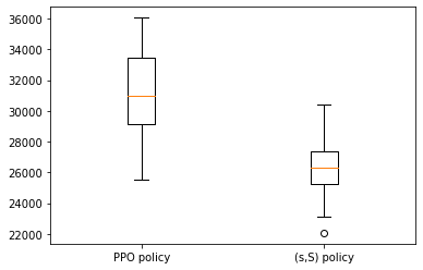
The average profit of the PPO policy across the 100 demand datasets is $31187.03, and the average profit of the (s,S) policy is $26390.87, which shows a 18.17% profit increase. The boxplot of the profits obtained by the PPO and (s,S) policies across the 100 demand datasets is shown below.
We have seen that the PPO policy outperforms the (s,S) policy with its current formulation. There may be some room to further improve its performance. For example, we can model actions as a continuous value x between [0,1]. Hence, the order quantity at each entity will be x*maximum order quantity. In my future articles, I may take a further step towards this direction to see how this approach would perform.
Thanks for reading!
Reinforcement Learning for Inventory Optimization Series II: An RL Model for A Multi-Echelon… was originally published in Towards Data Science on Medium, where people are continuing the conversation by highlighting and responding to this story.
...