

 800+ IT
News
als RSS Feed abonnieren
800+ IT
News
als RSS Feed abonnieren📚 Road Network Edge Matching With Triangles
💡 Newskategorie: AI Nachrichten
🔗 Quelle: towardsdatascience.com
Triangles have mighty properties for geospatial queries

Triangles are shapes with many practical geometric properties. In this article, I illustrate using such properties when performing opportunistic optimizations while solving a particular geospatial problem: the recovery of missing map-matched information.
I started exploring the Extended Vehicle Energy Dataset¹ (EVED) [1] a while ago to search for compelling geospatial data analysis opportunities in a city road network context. This dataset derives from a previous publication, the Vehicle Energy Dataset [2], and contains many enhancements, namely the vehicles’ map-matched GPS locations. The map-matching process snaps the original GPS locations to the most likely edges of the underlying road network.
Figure 1 below (taken from a previous article) illustrates how the map-matching process snaps the sampled GPS location to the most likely road network edge.
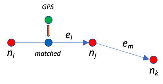
Unfortunately, the EVED dataset does not retain the underlying matched edge information; only the snapped location. With the missing edge information, we can make more inferences from the data, for example, to create a destination prediction model. Can we retrieve that information from the matched GPS locations?
The article authors used the Valhalla toolset to perform the map-matching operation using Open Street Map data for the underlying road network. Armed with this information, we can recover the missing mapped edge information using geospatial queries. We start by using one very well-known off-the-shelf tool: OSMnx. Our first task is to download the road network (aka graph).
Downloading the Road Network
To download and prepare the road network data, we need to use OSMnx’s facilities, as illustrated by the following code snippet².
def download_road_network(place_name, network_type='drive'):
    graph = ox.graph_from_place(place_name, network_type=network_type,
                                simplify=False)
    graph = ox.add_edge_speeds(graph)
    graph = ox.add_edge_travel_times(graph)
    graph = ox.bearing.add_edge_bearings(graph)
    return graph
We start by downloading a non-simplified graph to retain most of the node detail. Next, we add missing properties to the network, like edge speeds, travel times, and bearings (the angle measured in degrees from true North in the clockwise direction). The function returns the road network as a NetworkX [3] directed graph object that allows multiple edges between nodes.
road_network = download_road_network("Ann Arbor, Michigan, USA")Looking for Edges
As I mentioned, the EVED only contains the map-matched locations, not the edges themselves, and our job is to reconstruct this information. The map-matching process involves finding the network edges that maximize the matching probability between the observed route and the known road network. More concretely, the operation maps each GPS sample to the road network edge with the highest likelihood of representing the actual traveled route. The map-matching process projects the sampled GPS location, providing additional contextual information. The matched location belongs to the edge-defining geodesic, and we will see how to use this to our advantage in what follows.
The OSMnx Way
Let us now turn to OSMnx and discover a way to search for the road network edges that the map-matched locations belong to. Fortunately, the package implements functions to find the closest nodes and edges, which is where we will start.
The first step is to project the road network coordinates into UTM [4]. This conversion projects the spherical GPS coordinates to a local planar space where we can use regular geometry, and measurements are in meters.
network_utm = ox.projection.project_graph(road_network)
The function call above projects the road network coordinates to the UTM zone corresponding to the area’s center. We can now call OSMnx’s edge detection function using a coordinate pair from the database.
easting, northing, zone_num, zone_ltr = utm.from_latlon(42.287702, -83.707775)
edge_id = ox.distance.nearest_edges(network_utm, easting, northing)
Instead of a single location, the function supports latitude and longitude collections, returning the corresponding edge list. As for the above call, we can inspect its result using the following code:
network_utm[edge_id[0]][edge_id[1]][0]
The result is a Python dictionary containing the nearest edge properties, as depicted below.
{'osmid': 8723817,
 'oneway': False,
 'lanes': '2',
 'highway': 'tertiary',
 'reversed': True,
 'length': 116.428,
 'speed_kph': 48.3,
 'travel_time': 8.7,
 'bearing': 267.3,
 'name': 'Glazier Way',
 'maxspeed': '30 mph'}
Unfortunately, this function is slow. If we want to convert the whole EVED database to assign the closest edge to every point, we should try another way.
The Triangular Way
The solution I’m presenting in this section was the first to come to mind. As stated above, map-matched locations live in the edge’s geodesic line segment that connects the end nodes. This allows us to use triangle properties to find the best network edge for a specific point.
Before explaining further, I invite you to read an older article exploring triangle properties to perform high-speed geospatial queries.
Using the Triangle Inequality to Query Geographic Data
Here, I use an updated version of that article’s code to perform the basic search queries on the road network: the K nearest neighbors and the radius query. The updated code version uses Numba-based optimizations to improve its execution performance.
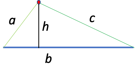
Besides using the triangle inequality to supercharge the geospatial queries, we will also use it to select the best edge for a given map-matched GPS sample. The idea is quite simple, and I illustrate it in Figure 2 below.
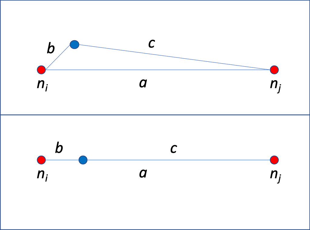
To match a given road network edge to a GPS point, we need to calculate the distances between said point to the nodes (b and c in Figure 2). The edge length (a) is a property of the downloaded road network data. We calculate the following ratio as a metric of fit.

The best-fitting road network edge will have the lowest possible value for this metric. But this is not the only criterion we must use, as the segment’s heading is also essential.
We query a network edge using the identifiers for the end nodes, and their order is important. By reversing the node identifiers in the network query, we get different properties for the reverse direction (if it exists), namely the calculated bearing or heading. Figure 4 below shows what these properties might look like.
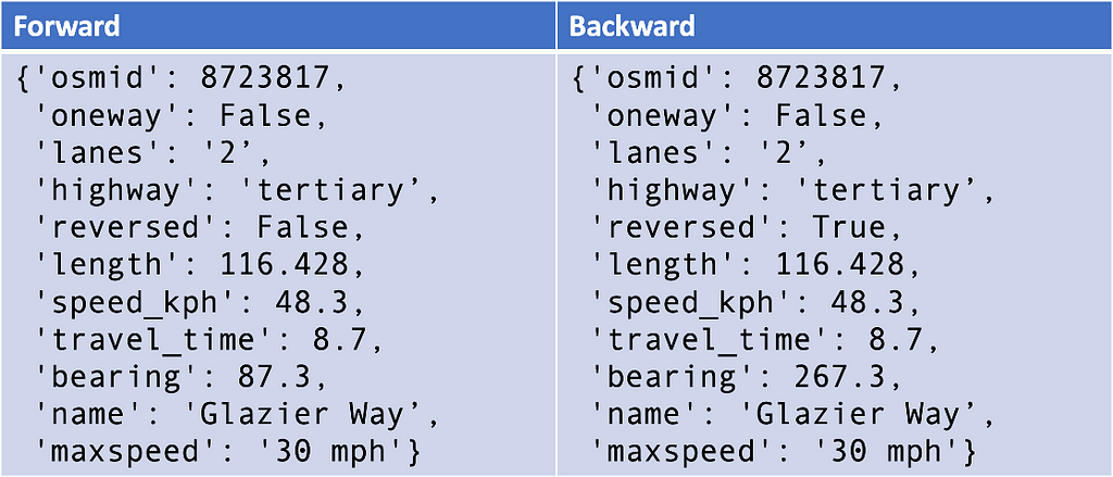
To correctly match the road network edge, we must also know the GPS heading or, as is the case, the inferred one. You can read the article below about calculating the EVED bearings from the matched GPS locations.
Travel Time Estimation Using Quadkeys
We are now ready to search for the best-fitting edge, but how should we search for it in an arbitrarily large road network? A brute-force approach would search through all available road segments, but that would not be a good use of computing power as we can do much better. We can select a small set of nearby candidates and then search within those only.
The criterion for selecting this candidate set is straightforward — we will use a radius query from the input GPS location. The radius comprises two parts, the smallest distance from the query point to the network and the maximum road segment length. By adding these two distances, we obtain a radius where we are sure that the closest edge nodes will reside. Figure 5 below illustrates this concept.
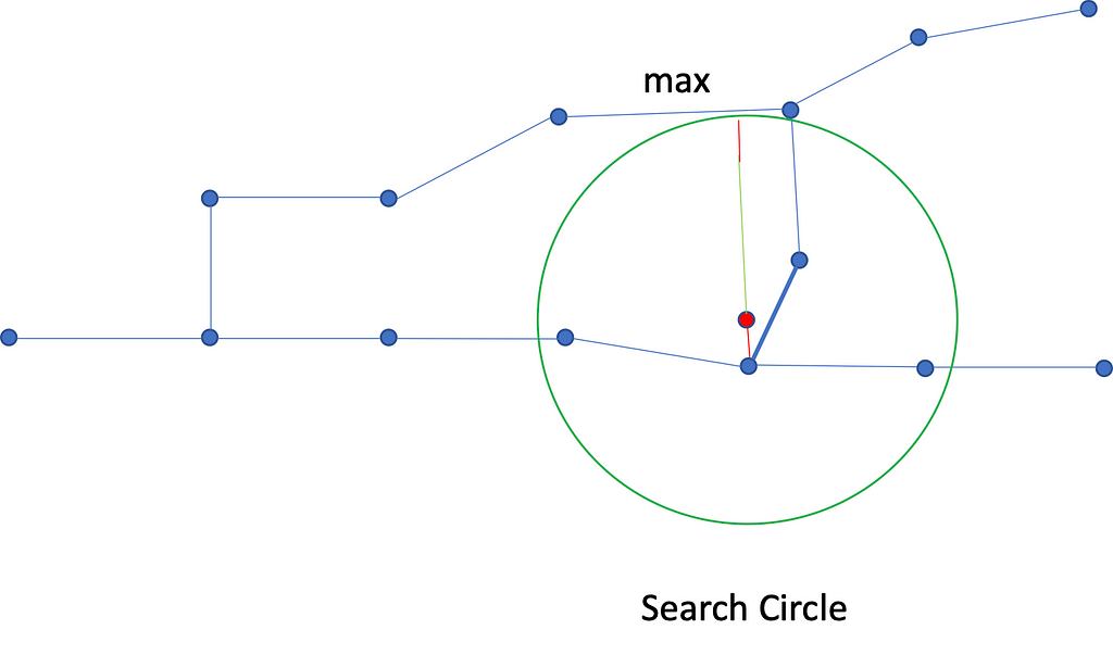
Once we have determined the candidate node set, we only consider the existing links within the search radius.
Let’s see what the code looks like. We start with the class declaration that handles the road network:
class RoadNetwork(object):

    def __init__(self, graph, projected=False):
        self.graph = graph
        self.projected = projected
        self.max_edge_length = max([graph[e[0]][e[1]][0]["length"] \
                                    for e in graph.edges])
        self.ids, self.locations = self.get_locations()
        self.geo_spoke = GeoSpoke(self.locations)
# more...
To initialize this class, we call the function that downloads and prepares the OSM road network and feeds its result as the constructor parameter. The constructor then collects all the locations and passes them to the indexer object, described in the previously-mentioned article. Note that we will not need to project any coordinates for this method.
The function that collects the geospatial coordinates is simple enough:
    def get_locations(self):
        latitudes = []
        longitudes = []
        ids = []
        for n in self.graph.nodes:
            ids.append(n)
            node = self.graph.nodes[n]
            longitudes.append(node['x'])
            latitudes.append(node['y'])

        locations = np.array(list(zip(latitudes, longitudes)))
        return np.array(ids), locations
# more...
Now, we can get to the algorithm’s core, the query process itself. For each query point, we want to select the most likely road network nodes that might delimit the edge’s geodesic segment. The function below takes location coordinates and finds the road network edge with the minimal value for the fit metric (Figure 3).
def get_matching_edge(self, latitude, longitude, bearing=None):
    loc = np.array([latitude, longitude])
    _, r = self.geo_spoke.query_knn(loc, 1)
    radius = self.max_edge_length + r[0]
    node_idx, dists = self.geo_spoke.query_radius(loc, radius)
    nodes = self.ids[node_idx]
    distances = dict(zip(nodes, dists))
    adjacent_set = set()
    graph = self.graph

    best_edge = None
    for node in nodes:
        if node not in adjacent_set:
            adjacent_nodes = np.intersect1d(np.array(graph.adj[node]),
                                            nodes, assume_unique=True)

            adjacent_set.update(adjacent_nodes)
            for adjacent in adjacent_nodes:
                edge_length = graph[node][adjacent][0]['length']
                ratio = (distances[node] + distances[adjacent]) / \
                        edge_length
                if best_edge is None or ratio < best_edge[2]:
                    best_edge = (node, adjacent, ratio)


        if bearing is not None:
            best_edge = fix_edge_bearing(best_edge, bearing, graph)
    return best_edge
The code starts by finding the closest road network node and its distance. It then calculates the search radius by adding this distance to the largest road network edge length. The ensuing radius query returns the set of candidate nodes and their distances to the query location. We now use the node identifiers as keys to a dictionary of the distances for faster retrieval.
The main loop iterates through the candidate nodes and finds the adjacent nodes within the query radius that still need to be iterated. Finally, the code calculates the fit ratio and retains the best road network edge.
But there is a final test in the returned road network edge: its orientation. We can go about this if we have the sample GPS heading. As I previously explained, we have the inferred heading value that we can use. You can see this in the final part of the code, which only works if you provide a bearing and if the reverse edge exists. The function that fixes the edge bearing is shown below.
def fix_edge_bearing(best_edge, bearing, graph):
    if (best_edge[1], best_edge[0], 0) in graph.edges:
        bearing0 = radians(graph[best_edge[0]][best_edge[1]][0]['bearing'])
        bearing1 = radians(graph[best_edge[1]][best_edge[0]][0]['bearing'])
        gps_bearing = radians(bearing)
        if cos(bearing1 - gps_bearing) > cos(bearing0 - gps_bearing):
            best_edge = (best_edge[1], best_edge[0], best_edge[2])
    return best_edge
You can test this code using the accompanying Jupyter notebook in the GitHub repository. In my MacBook Pro, this code offers a performance improvement of over three times over the OSMnx approach.
The Distance Way
One might argue that the previous arrangement performs better under rigorous assumptions, namely that the query locations already live over the road segment’s geodesic. What if that is not the case? Can we develop a more general approach based on the same search principles? We can! But we must assume that distances are small³, so we do not have to project the coordinates, which is, fortunately, the case.
Instead of using the aforementioned triangle ratio metric, we can calculate the distance between the GPS location and any nearby road segment without requiring any geospatial projection (like UTM mentioned above). Again, we rely on triangle properties to calculate the distance using two alternate methods of computing the triangle area and other triangle inequalities [5].
When calculating the distance from a given point to a line segment, we have two cases to consider, when we can make an orthogonal projection of the point to the segment and when we cannot. Let us visualize the first case in Figure 6 below.
For this case, our unknown is the triangle’s height, which is the shortest distance from the point to the road segment. So how do we calculate it? One of the best-known triangle area formulas uses that quantity and is shown in Figure 7 below.

If the area is known, we can quickly derive the height using simple algebra. Can we calculate the triangle’s area using just the side lengths?
Another probably less well-known triangle area formula got its name from Heron of Alexandria [6], who proved it “first.” Interestingly, this formula only depends on things that we already know — the size of the triangle sides. This formula has several forms, and the most famous is probably the one in Figure 8 below.

Using this formula, we can compute the triangle area and use it in the previous one to get the distance from the sample point to the segment. Unfortunately, this formulation is known to have numerical stability issues, especially when applied to very “flat” triangles with very sharp angles. We will use a known stable alternative depicted in Figure 9 below.

What happens when we cannot orthogonally project the query point to the road segment? We visualize this situation if Figure 10 below.
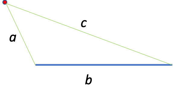
In this situation, we have it easy as the distance is already calculated. But how do we know the geometry using side lengths only? One observation we can make distinguishes the triangles in Figure 6 and Figure 10. In Figure 6, the angles that segments “a” and “c” make with “b” are both acute, while in Figure 10, one of them is obtuse (larger than 90 degrees).
Fortunately, geometry helps us with a different set of triangle inequalities that help us determine if an internal triangle angle is either acute, obtuse, or straight. In the case of Figure 9, we have c² > a² + b². In the symmetric case, where the opposing angle is obtuse, we would have a² > b² + c². These two tests tell the two situations apart and are very fast to execute.
The code below illustrates the query that uses distances instead of a simple fitness ratio.
def get_nearest_edge(self, latitude, longitude, bearing=None):
    best_edge = None
    adjacent_set = set()
    graph = self.graph

    loc = np.array([latitude, longitude])
    _, r = self.geo_spoke.query_knn(loc, 1)
    radius = self.max_edge_length + r[0]
    node_idx, dists = self.geo_spoke.query_radius(loc, radius)
    nodes = self.ids[node_idx]
    distances = dict(zip(nodes, dists))

    for node in nodes:
        if node not in adjacent_set:
            adjacent_nodes = np.intersect1d(np.array(graph.adj[node]),
                                            nodes, assume_unique=True)

            adjacent_set.update(adjacent_nodes)
            for adjacent in adjacent_nodes:
                a = distances[node]
                b = graph[node][adjacent][0]['length']
                c = distances[adjacent]

                a2, b2, c2 = a * a, b * b, c * c

                if c2 > a2 + b2 or a2 > b2 + c2:
                    distance = min(a, c)
                else:
                    area = heron_area(a, b, c)
                    distance = area * 2.0 / b

                if best_edge is None or distance < best_edge[2]:
                    best_edge = (node, adjacent, distance)

    if bearing is not None:
        best_edge = fix_edge_bearing(best_edge, bearing, graph)
    return best_edge
Finally, the following function calculates Heron’s formula from three arbitrary triangle side lengths. Note how the code starts by sorting the side lengths appropriately.
@njit()
def heron_area(a, b, c):
    c, b, a = np.sort(np.array([a, b, c]))
    return sqrt((a + (b + c)) *
                (c - (a - b)) *
                (c + (a - b)) *
                (a + (b - c))) / 4.0
Let’s see if all this effort was called for.
Performance
I obtained the performance results below using a 16-inch MacBook Pro from 2019 with a 2.6 GHz 6-Core Intel Core i7 CPU, 32 GB RAM, and Ventura 13.0. All three methods queried the same 868-point trajectory taken from the EVED.
In Figure 11 below, you can see the benchmark results of the three algorithms in the order I presented them in this article.
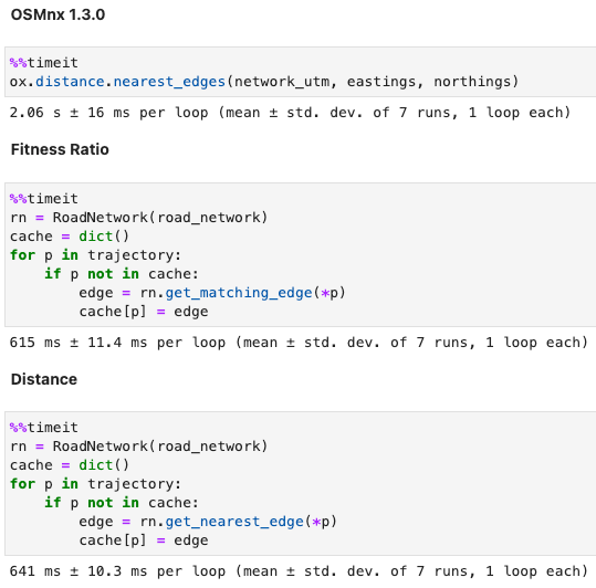
As you can see, I am using a cache to handle the duplicates and avoid unnecessary processing. This might provide an unfair advantage over the OSMnx algorithm, and to clarify, I decided to run the same benchmark with the set of 203 unique locations from the same path. The results are displayed below in Figure 12.
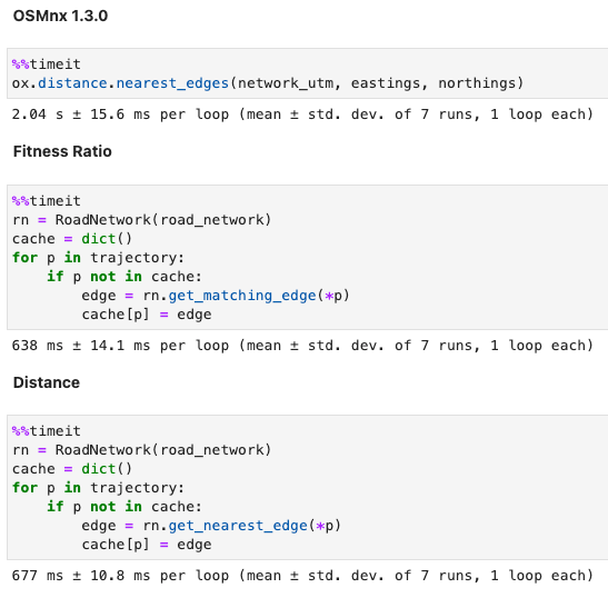
Note that for OSMnx versions before 1.3.0, the performance difference was dramatically worse.
We have used our triangle properties and found a speedy algorithm to match edges. Still, I should conduct further tests to investigate edge cases and larger road networks to ensure this is a solid algorithm.
Conclusion
In this article, I developed a fast algorithm to search for the missing map-matched edges of the EVED locations. By assuming that these locations lie on a road network edge geodesic, I developed a fast fit metric using the triangle inequality property. Next, I enriched the algorithm to use the geometric concept of the distance of a point to a line segment. I used more triangle properties and inequalities to consider side lengths only. Finally, I benchmarked the solution and confirmed the performance improvement of the new algorithms over the OSMnx one.
Finally, let me stress that the performance gains result from the strong assumptions I could make from the problem definition. The performance of this algorithm degrades by increasing the search radius, which is highly dependent on the road network structure, and node density.
Please get the code from the GitHub repository.
Notes
- The original paper authors licensed the dataset under the Apache 2.0 License (see the VED and EVED GitHub repositories). Note that this also applies to derivative work.
- I licensed all the code in this article and the accompanying GitHub repository using the MIT License.
- We are dealing with relatively small distances with this dataset. The maximum road segment length for the downloaded data is less than 600 meters (0.37 miles or 1968 feet). You can probably use larger distances safely without a significant error, but I suggest checking whether the incurred error is acceptable.
References
[1] Zhang, S., Fatih, D., Abdulqadir, F., Schwarz, T., & Ma, X. (2022). Extended vehicle energy dataset (eVED): an enhanced large-scale dataset for deep learning on vehicle trip energy consumption. arXiv. https://doi.org/10.48550/arXiv.2203.08630
[2] Oh, G. S., Leblanc, D. J., & Peng, H. (2019). Vehicle Energy Dataset (VED), A Large-scale Dataset for Vehicle Energy Consumption Research. arXiv. https://doi.org/10.48550/arXiv.1905.02081
[3] Aric A. Hagberg, Daniel A. Schult, and Pieter J. Swart, “Exploring network structure, dynamics, and function using NetworkX,” in Proceedings of the 7th Python in Science Conference (SciPy2008), Gäel Varoquaux, Travis Vaught, and Jarrod Millman (Eds), (Pasadena, CA USA), pp. 11–15, Aug 2008
[4] Universal Transverse Mercator coordinate system. (2022, June 16). In Wikipedia. https://en.wikipedia.org/wiki/Universal_Transverse_Mercator_coordinate_system
[5] List of triangle inequalities. (2022, December 17). In Wikipedia. https://en.wikipedia.org/wiki/List_of_triangle_inequalities
[6] Heron’s formula. (2022, December 17). In Wikipedia. https://en.wikipedia.org/wiki/Heron%27s_formula
João Paulo Figueira works as a Data Scientist at tb.lx by Daimler Trucks and Buses in Lisbon, Portugal.
Road Network Edge Matching With Triangles was originally published in Towards Data Science on Medium, where people are continuing the conversation by highlighting and responding to this story.
...