

 800+ IT
News
als RSS Feed abonnieren
800+ IT
News
als RSS Feed abonnieren📚 The Kinetic Theory of Gases: Modeling the Dynamics of Ideal Gas Molecules
💡 Newskategorie: AI Nachrichten
🔗 Quelle: towardsdatascience.com
Statistical mechanics
Develop a framework to simulate and visualize molecular collisions, and extract thermodynamic insights using Python
Introduction
Imagine someone constantly throwing a ball at your head. Depending upon the size and mass of the ball, you may feel anything between mild annoyance and unbearable agony. And yet, there are countless such “balls” colliding with, not only your head, but your whole body every instant and you do not feel a thing. Nitrogen, oxygen, and water molecules in the air are in constant random motion around you, even when the air appears to be stationary. The result of the collisions of these molecules with you is that air exerts a certain pressure on you (termed atmospheric pressure). Since we are “used to” the atmospheric pressure, it does not feel like anything out of the ordinary, but if you are ever in an airplane or a hyperbaric chamber, where the pressure deviates from the atmospheric pressure, you may notice different sensations, like ear-popping, that are your body’s responses to changes in pressure.
A macroscopic understanding of pressure, and how it varies with the volume that a gas occupies was given by Robert Boyle in the 17th century, that is commonly termed as Boyle’s law. However, it was only a century later that a qualitative molecular picture was provided by Daniel Bernoulli to explain pressure, and also relate it to the temperature and kinetic energy of molecules. This “kinetic theory,” however, did not find much acceptance until, in the 19th century, James Clerk Maxwell, building on the work of Rudolf Clausius, formalized it in terms of a statistical law and Ludwig Boltzmann illuminated its relationship with entropy, leading to the formulation of the Maxwell-Boltzmann distribution of velocities of molecules in a gas. This eventually led to the development of a detailed theoretical treatment of gases from the molecular point of view, which was consistent with the well-understood macroscopic view.
In this article, we will try to link the molecular picture of gases with its macroscopic properties — that is, pressure, volume, and temperature — by performing a series of numerical simulations using Python.
Theoretical background
Kinetic theory of gases
The kinetic theory of gases is a model that describes a gas in terms of molecules that are in constant, random motion.
- Molecules travel in straight lines until they are interrupted by elastic collisions with other molecules or the walls of the container. Elasticity implies that no kinetic energy is lost in collisions.
- Molecules do not “interact” with each other, that is, they do not exert any attractive or repulsive intermolecular forces.
- The volume occupied by the molecules themselves is considered to be negligible compared to the volume occupied by the gas.
If molecules following these rules are sampled and their velocities measured, they will conform to the Maxwell-Boltzmann distribution. The temperature of the gas is actually a property that we define based on the shape of the distribution. The higher the average kinetic energy is (or the flatter the distribution is), the higher the temperature of the gas is, and vice versa. It does not make sense to define a temperature of an individual molecule; rather, it is an averaged property of a collection of molecules.
Note that the kinetic theory of gases is a model, it is not necessarily a true reflection of reality (as is the case with all scientific models). Molecular collisions are not strictly elastic, and molecules do have short-range interactions. However, a model with these relatively simple assumptions is able to replicate the properties of an ideal gas very well, which is a very useful macroscopic model to predict the behavior of gases under various conditions.
Ideal gas law
An ideal gas is a hypothetical gas whose properties are related to each other through a simple equation-of-state, called the ideal gas law.

Here P refers to the pressure of the gas, V refers to the volume of the container, T is the temperature, and n is the number of moles of the gas. If any of these three quantities are held constant, the fourth does not change as well, and this is reflected through R, which is the universal gas constant. The ideal gas law is an accurate model for a gas that is at a high temperature or low pressure, since most of the assumptions of the kinetic theory of gases are true in these regimes.
We will test two relationships based on the ideal gas law with our model.
- At a constant temperature and number of moles, the pressure is inversely proportional to the volume.
- At a constant volume and number of moles, the pressure is directly proportional to the temperature.
The former is referred to as Boyle’s law and the latter is referred to as Gay-Lussac’s law, both named after researchers that first discovered the relationships between these variables through experiments.
Setting up the computational model
To simulate the motion of molecules according to the kinetic theory of gases, we need to set up a dynamic n-body simulation with collisions. Note that the objective of this article is to produce a simulation for pedagogical purposes. Therefore, the code is set up to maximize understanding, not execution speed.
Defining molecular properties
We start by importing all the required modules.
import os
import sys
import time
import numpy as np
import scipy as sci
import matplotlib.pyplot as plt
from matplotlib.animation import FuncAnimation
First, we will define a class called Molecule. Objects of this class will store properties such as the masses, positions and velocities of molecules in the simulation. We also define an attribute called color, that may be used to distinguish between different gases and set the color of the points in the animation.
class Molecule(object):
    #Constructor
    def __init__(self,molecule,position,velocity,mass,color="black"):
        self.molecule=molecule
        self.position=np.array([x_i for x_i in position])
        self.velocity=np.array([v_i for v_i in velocity])
        self.mass=mass
        self.color=color

    #Setters for position, velocity, mass and color
    def set_position(self,position):
        self.position=np.array([x_i for x_i in position])

    def set_velocity(self,velocity):
        self.velocity=np.array([v_i for v_i in velocity])

    def set_color(self,color):
        self.color=color

    def set_mass(self,mass):
        self.mass=mass

    #Getters for position, velocity, mass and color
    def get_position(self):
        return self.position

    def get_velocity(self):
        return self.velocity

    def get_color(self):
        return self.color

    def get_mass(self):
        return self.mass
Adding molecules to a box
Next, we create a Simulation class and define key input parameters, such as the dimensions of the simulation box, that ultimately control the volume of the gas. We also initialize variables for bookkeeping, such as for the wall momentum, that will allow us to calculate pressure.
class Simulation(object):
    #Constructor
    def __init__(self,name,box_dim,t_step,particle_radius):
        #Set simulation inputs
        self.name=name #Name of the simulation
        self.box_dim=[x for x in box_dim] #Dimensions of the box
        self.t_step=t_step #Timestep
        self.particle_radius=particle_radius #Radius of the particles

        #Calculate volume and number of dimensions
        self.V=np.prod(self.box_dim) #Area/Volume of the box
        self.dim=int(len(box_dim)) #Number of dimensions (2D or 3D)

        #Initialize paramters
        self.molecules=[] #Create empty list to store objects of class Molecule
        self.n_molecules=0 #Create variable to store number of molecules
        self.wall_collisions=0 #Create variable to store number of wall collisions
        self.wall_momentum=0 #Create variable to store net momentum exchanged with wall
To add molecules, we first need to initialize their positions and velocities. For both, we can define functions that create arrays of values based on a distribution input by the user. Note that it does not matter what distributions the initialized positions and velocities follow (as long as there is nothing unphysical, like a molecule outside the box). We shall see that the velocities eventually follow the same distribution.
    #Still in Simulation class
    def _generate_initial_positions(self,n,dist="uniform"):
            #Uniform distribution
            if dist=="uniform":
                _pos=np.random.uniform(low=[0]*self.dim,high=self.box_dim,size=(n,self.dim))

            #Store positions in temporary variable
            self._positions=_pos

    def _generate_initial_velocities(self,n,v_mean,v_std,dist="normal"):
        #Normal distribution with mean v_mean and std v_std
        if dist=="normal":
            self.v_mean=v_mean
            self.v_std=v_std
            _vel=np.random.normal(loc=v_mean,scale=v_std,size=(n,self.dim))

        #Uniform distribution with lower bound v_mean and higher bound v_std
        if dist=="uniform":
            self.v_mean=v_mean
            self.v_std=v_std
            _vel=np.random.uniform(low=v_mean,high=v_std,size=(n,self.dim))

        #All velocities equal to v_mean
        if dist=="equal":
            self.v_mean=v_mean
            self.v_std=v_std
            _vel=v_mean*np.ones((n,self.dim))

        #Randomly switch velocities to negative with probability 0.5
        for i in range(_vel.shape[0]):
            for j in range(_vel.shape[1]):
                if np.random.uniform() > 0.5:
                    _vel[i,j]=-_vel[i,j]

        #Store velocities in temporary variable
        self._velocities=_vel
It is time to add the molecules to the box. We call the two previously defined functions to generate arrays of initial positions and velocities, create objects of the Molecule class, and assign them to the objects.
    #Still in Simulation class
    def add_molecules(self,molecule,n,v_mean,v_std,pos_dist="uniform",v_dist="normal",color="black"):
        #Generate initial positions and velocities
        self._generate_initial_positions(n,dist=pos_dist)
        self._generate_initial_velocities(n,v_mean,v_std,dist=v_dist)

        #Initialize objects of class Molecule in a list (set mass to 1 as default)
        _add_list=[Molecule(molecule,position=self._positions[i,:],velocity=self._velocities[i,:],color=color,mass=1) for i in range(n)]
        self.molecules.extend(_add_list)
        self.n_molecules+=len(_add_list)
Finally, we write a function for general bookkeeping, that is, to make matrices to store the position and velocity vectors as well as their magnitudes. We also make a distance matrix, that stores the distance between every two molecules. This will come in handy to detect collisions.
    #Still in Simulation class
    def make_matrices(self):
        #Make empty matrices to store positions, velocities, colors, and masses
        self.positions=np.zeros((self.n_molecules,self.dim))
        self.velocities=np.zeros((self.n_molecules,self.dim))
        self.colors=np.zeros(self.n_molecules,dtype="object")
        self.masses=np.zeros(self.n_molecules)

        #Iterate over molecules, get their properties and assign to matrices
        for i,m in enumerate(self.molecules):
            self.positions[i,:]=m.get_position()
            self.velocities[i,:]=m.get_velocity()
            self.colors[i]=m.get_color()
            self.masses[i]=m.get_mass()

        #Make vectors with magnitudes of positions and velocities
        self.positions_norm=np.linalg.norm(self.positions,axis=1)
        self.velocities_norm=np.linalg.norm(self.velocities,axis=1)

        #Make distance matrix
        self.distance_matrix=np.zeros((self.n_molecules,self.n_molecules))
        for i in range(self.distance_matrix.shape[0]):
            for j in range(self.distance_matrix.shape[1]):
                self.distance_matrix[i,j]=np.linalg.norm(self.positions[i,:]-self.positions[j,:])

        #Set diagonal entries (distance with itself) to a high value
        #to prevent them for appearing in the subsequent distance filter
        np.fill_diagonal(self.distance_matrix,1e5)
Detecting and handling collisions
Here, we come to the meat of the simulation, that is, modeling the dynamics of the molecules. Collision physics are defined for a 2D plane, but extension to a 3D box is possible with minor changes. We define a function that goes through a three-item checklist:
- Check if there are molecule-molecule collisions and if yes, update velocities accordingly
- Update positions of the molecules based on their velocities
- Check if there are molecule-wall collisions and if yes, update velocities and wall momentum accordingly
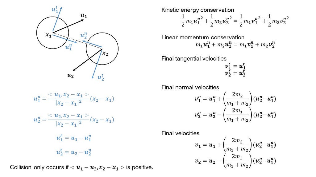
To filter molecules that are close enough to collide, we scour the distance matrix and return the pairs of indices of molecules that have distances less than the sum of their radii. It is possible for molecules to be within this cutoff, and yet be departing away from each other. So, we apply another criterion (see Figure 1) to investigate whether molecules are approaching each other. If they are, we update their velocities based on the equations given in Figure 1. We arrive at these equations by conserving the kinetic energies and the linear momenta (along the collision axis) of the molecules.
Updating the positions of the molecules is quite simple. We add the product of the velocity vector and the timestep to the previous position to get the new position. To identify collisions with the walls, we simply check if the new position of a molecule exceeds either the lower or upper bounds of the dimensions of the box. If it does, we change the sign of the velocity normal to the wall, and set the new position based on this velocity. Further, we add twice the magnitude of this velocity to the variable tracking the momentum exchanged with the wall.
    #Still in Simulation class
    def update_positions(self):
        #1: Check molecule collisions

        #Find molecule pairs that will collide
        collision_pairs=np.argwhere(self.distance_matrix < 2*self.particle_radius)

        #If collision pairs exist
        if len(collision_pairs):

            #Go through pairs and remove repeats of indices
            #(for eg., only consider (1,2), remove (2,1))
            pair_list=[]
            for pair in collision_pairs:
                add_pair=True
                for p in pair_list:
                    if set(p)==set(pair):
                        add_pair=False
                        break
                if add_pair:
                    pair_list.append(pair)

            #For every remaining pair, get the molecules, positions, and velocities
            for pair in pair_list:
                m_1=self.molecules[pair[0]]
                m_2=self.molecules[pair[1]]

                x_1=m_1.get_position()
                x_2=m_2.get_position()

                u_1=m_1.get_velocity()
                u_2=m_2.get_velocity()

                #Check if molecules are approaching or departing
                approach_sign=np.sign(np.dot(u_1-u_2,x_2-x_1))
                #If molecules are approaching
                if approach_sign == 1:
                    #Get masses
                    ms_1=m_1.get_mass()
                    ms_2=m_2.get_mass()

                    #Calculate final velocities
                    v_1=u_1 - 2*ms_2/(ms_1 + ms_2) * (np.dot(u_1-u_2,x_1-x_2)/np.linalg.norm(x_1-x_2)**2) * (x_1 - x_2)
                    v_2=u_2 - 2*ms_1/(ms_1 + ms_2) * (np.dot(u_2-u_1,x_2-x_1)/np.linalg.norm(x_2-x_1)**2) * (x_2 - x_1)

                    #Update velocities of the molecule objects
                    m_1.set_velocity(v_1)
                    m_2.set_velocity(v_2)

        #2: Update positions

        #Iterate over all the molecule objects
        for i,m in enumerate(self.molecules):
            #Get the position, velocity, and mass
            _x=m.get_position()
            _v=m.get_velocity()
            _m=m.get_mass()

            #Calculate new position
            _x_new=_x + _v * self.t_step

            #3: Check wall collisions

            #Check collisions with the top and right walls
            _wall_diff=_x_new - np.array(self.box_dim)
            #If wall collisions present
            if _wall_diff[_wall_diff>=0].shape[0] > 0:
                #Increment collision counter
                self.wall_collisions+=1
                #Check whether collision in x or y direction
                _coll_ind=np.argwhere(_wall_diff>0)
                #For component(s) to be reflected
                for c in _coll_ind:
                    #Reflect velocity
                    _v[c]=-_v[c]
                    #Increment wall momentum
                    self.wall_momentum+=2*_m*np.abs(_v[c])
                #Update velocity
                m.set_velocity(_v)
                #Update position based on new velocity
                _x_new=_x + _v * self.t_step

            #Check collisions with the bottom and left walls
            if _x_new[_x_new<=0].shape[0] > 0:
                #Increment collision counter
                self.wall_collisions+=1
                #Check whether collision in x or y direction
                _coll_ind=np.argwhere(_x_new<0)
                #For component(s) to be reflected
                for c in _coll_ind:
                    #Reflect velocity
                    _v[c]=-_v[c]
                    #Increment wall momentum
                    self.wall_momentum+=2*_m*np.abs(_v[c])
                #Update velocity
                m.set_velocity(_v)
                #Update position based on new velocity
                _x_new=_x + _v * self.t_step

            #Update position of the molecule object
            m.set_position(_x_new)

        #Construct matrices with updated positions and velocities
        self.make_matrices()
That’s it, the hard part is done! Finally, we need to write a function to run the simulation. This involves calling the functions that we have defined previously in a loop that runs for a specified number of iterations, calculated based on the specified simulation time and time step.
    #Still in Simulation class
    def safe_division(self,n,d):
        if d==0:
            return 0
        else:
            return n/d

    def run_simulation(self,max_time):
        #Print "Starting simulation"
        print("Starting simulation...")

        #Make matrices
        self.make_matrices()

        #Calculate number of iterations
        self.max_time=max_time
        self.n_iters=int(np.floor(self.max_time/self.t_step))

        #Make tensors to store positions and velocities of all molecules at each timestep f
        self.x_dynamics=np.zeros(((self.n_molecules,self.dim,self.n_iters)))
        self.v_dynamics=np.zeros((self.n_molecules,self.n_iters))

        #In each iteration
        for i in range(self.n_iters):
            #Save positions and velocities to the defined tensors
            self.x_dynamics[:,:,i]=self.positions
            self.v_dynamics[:,i]=self.velocities_norm

            #Calculate rms velocity
            self.v_rms=np.sum(np.sqrt(self.velocities_norm**2))/self.velocities_norm.shape[0]

            #Print current iteration information
            _P=self.safe_division(self.wall_momentum,i*self.t_step*np.sum(self.box_dim))
            print("Iteration:{0:d}\tTime:{1:.2E}\tV_RMS:{2:.2E}\tWall Pressure:{3}".format(i,i*self.t_step,self.v_rms,_P))

            #Call the update_positions function to handle collisions and update positions
            self.update_positions()

        #Caclulate final pressure
        self.P=self.wall_momentum/(self.n_iters*self.t_step*np.sum(self.box_dim))
        print("Average pressure on wall: {0}".format(self.P))
        return self.P
That concludes the code involving the physics of the simulation. Running a simulation is no fun, however, if you cannot visualize it. Let’s utilize matplotlib to create an animation of the simulation.
Animating the simulation box
We start by writing a function to create a figure with an aspect ratio that is consistent with the provided dimensions of the box.
    #Still in Simulation class
    def create_2D_box(self):
        fig=plt.figure(figsize=(10,10*self.box_dim[1]/self.box_dim[0]),dpi=300)
        return fig
We will use the Animation module in matplotlib to make the animation. To utilize that, we need to define a function that takes the iteration number (frame) as input and creates a plot. This function is then provided as an argument to the FuncAnimation function in the Animation module.
    #Still in Simulation class
    def show_molecules(self,i):
        #Clear axes
        plt.cla()

        #Plot a line showing the trajectory of a single molecule
        plt.plot(self.x_dynamics[0,0,:i+1],self.x_dynamics[0,1,:i+1],color="red",linewidth=1.,linestyle="-")

        #Plot a single molecule in red that is being tracked
        plt.scatter(self.x_dynamics[0,0,i],self.x_dynamics[0,1,i],color="red",s=20)

        #Plot the rest of the molecules
        plt.scatter(self.x_dynamics[1:,0,i],self.x_dynamics[1:,1,i],color=self.colors[1:],s=20)

        #Remove ticks on the plot
        plt.xticks([])
        plt.yticks([])

        #Set margins to 0
        plt.margins(0)

        #Set the limits of the box according to the box dimensions
        plt.xlim([0,self.box_dim[0]])
        plt.ylim([0,self.box_dim[1]])

    def make_animation(self,filename="KTG_animation.mp4"):
        #Call the function to create the figure
        fig=self.create_2D_box()

        #Create the animation
        anim=FuncAnimation(fig,self.show_molecules,frames=self.n_iters,interval=50,blit=False)

        #Save animation as a file
        anim.save(filename,writer="ffmpeg")
There is another animation that we can make, showing histograms of velocities every iteration. This will allow us to observe the convergence of the velocity distribution to a Maxwell-Boltzmann distribution.
    #Still in Simulation class
    def plot_hist(self,i):
        #Clear axes
        plt.cla()

        #Make histogram
        plt.hist(self.v_dynamics[:,i],density=True,color="plum",edgecolor="black")

        #Define axis limits
        plt.xlim([0,3])
        plt.ylim([0,3])

    def make_velocity_histogram_animation(self,filename="KTG_histogram.mp4"):
        #Create empty figure
        fig=plt.figure(figsize=(5,5),dpi=500)

        #Create animation
        anim_hist=FuncAnimation(fig,self.plot_hist,frames=self.n_iters,interval=50,blit=False)

        #Save animation
        anim_hist.save(filename,writer="ffmpeg")
Running the simulation
It’s time to reap the rewards of our hard work. The effort spent in writing the code in an object-oriented fashion will pay off now, since we now have a generalized solver and can run simulations with different input parameters with just a few lines of code.
if __name__=="__main__":
    #Create simulation object and define input parameters
    sim=Simulation(name="kinetic_theory_simulation",box_dim=[1.0,1.0],t_step=1e-2,particle_radius=1e-2)

    #Add N2 molecules to the box
    sim.add_molecules("N2",n=100,v_mean=1.0,v_std=0.2,v_dist="normal")

    #Run the simulation and store the pressure output in P
    P=sim.run_simulation(15)

    #Make the box animation
    sim.make_animation()

    #Make the histogram animation
    sim.make_velocity_histogram_animation()
Animations of the simulation box and velocity histogram corresponding to the above simulation are shown below. In the first graphic, the movements of the molecules in the box, along with collisions, are shown, and the trajectory of one selected molecule is highlighted in red, for illustrative purposes. In the second graphic, the histogram of velocities of all the molecules in the box is shown at each iteration, and it is clear from the animation that the initial distribution, which is Gaussian (as specified), changes to a distribution that has a narrower left tail and broader right tail, mimicking the characteristics of a Maxwell-Boltzmann distribution. More rigorous statistical tests can be used to support this quantitatively.
https://medium.com/media/6b3e9620534983fba3b5f2be0a9a48c0/hrefhttps://medium.com/media/3f42400b008d783aaab5e0a4c2f33dbc/hrefExtracting thermodynamic insights
We return to the ideal gas law that relates various thermodynamic variables to each other. As mentioned previously, we test two relationships — pressure against volume and pressure against temperature. We keep the number of molecules in the box constant for all the subsequent simulations. The three variables — pressure, volume, and temperature — are calculated as follows: the pressure is the net momentum exchanged with the walls during the entire simulation divided by the product of the total simulation time and perimeter of the box. The volume is defined as the product of the length and breadth of the box (technically it is the area, since we are working in two dimensions, but the insights can be generalized easily to three dimensions).
Defining the temperature is trickier — since the temperature is proportional to the average kinetic energy of the molecules in the box, we consider the square of the mean velocity of the initial distribution to be a proxy for temperature. To remove any stochasticity from this estimate, the initial velocities assigned to the molecules in these simulations are set to a single specified value. For instance, if the specified value is 1 m/s, the initial velocities of all molecules are either +1 m/s or -1 m/s. This ensures that the initial total kinetic energy has a well-defined value that remains the same across all simulations that have the same temperature. Essentially, when the temperatures in two simulations are same, their initial total kinetic energies are same, which should ensure that the average kinetic energy during the simulation is also the same.
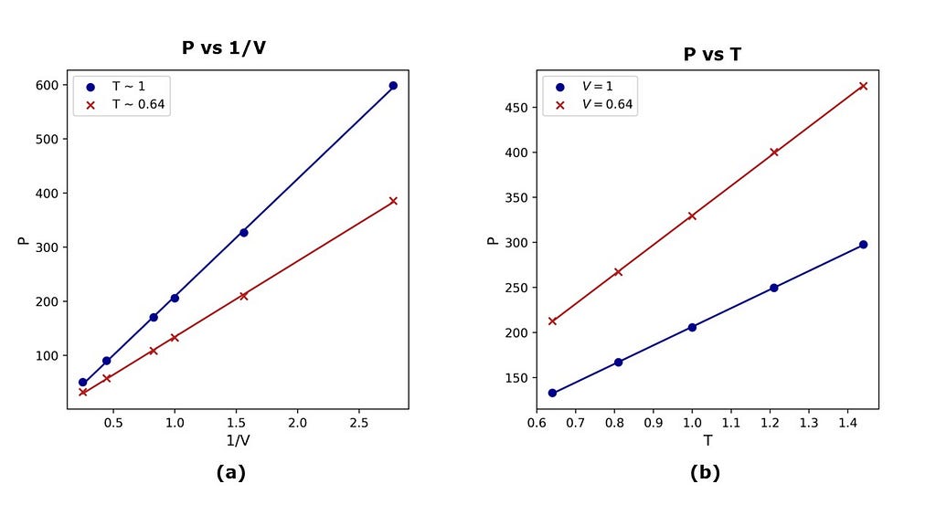
The results of the simulations are given in Figure 2. The average pressure on the walls of the box increases linearly with an increase in the inverse of the volume at a constant temperature (see Figure 2a). The slope of each isotherm is proportional to the temperature, consistent with the ideal gas law. In a second set of simulations, it is observed that the pressure increases linearly with an increase in the temperature at a constant volume (see Figure 2b). In this case, the slope of each isochore is inversely proportional to the volume, also consistent with the ideal gas law. Therefore, these microscopic simulations are able to reproduce trends in thermodynamic variables that are consistent with macroscopic theories like the ideal gas law.
Conclusions
The n-body simulation presented in this article is an example of a simple molecular dynamics simulation without any interactive forces. This is, of course, a gross oversimplification of how molecules behave and interact with each other but, as we have seen, it is sufficient to predict properties of an ideal gas. However, the ideal gas assumption is rarely used for calculating properties of gases for engineering applications, like the expansion of steam in a steam turbine. More complex equation-of-state models that include interactions between molecules are required to accurately model such processes. Adding short-range interactions between molecules in this code can lead to better reproduction of trends predicted by such models for real gases. Further, the usage of potentials like Lennard-Jones and addition of thermostats can allow prediction of properties for liquids as well.
The complete code for this simulation is available on GitHub. If you have any questions, suggestions, or comments, please feel free to reach out to be on email or Twitter.
To read more about the history of the kinetic theory of gases, refer to:
S. Brush, History of the Kinetic Theory of Gases (2004)
The Kinetic Theory of Gases: Modeling the Dynamics of Ideal Gas Molecules was originally published in Towards Data Science on Medium, where people are continuing the conversation by highlighting and responding to this story.
...