

 800+ IT
News
als RSS Feed abonnieren
800+ IT
News
als RSS Feed abonnieren📚 Analyzing Chess960 Data
💡 Newskategorie: AI Nachrichten
🔗 Quelle: towardsdatascience.com
Using more than 14M Chess960 games to find if there’s a variation that’s better than the others
In this post, I analyze all the available Chess960 games played in Lichess. With this information, and using Bayesian A/B testing, I show that there are no starting positions that favor any of the players more than other positions.
The original post was published here. All the images and plots, unless stated otherwise, are by the author.

Introduction
The World Fischer Random Chess Championship recently took place in Reykjavik, with GMHikaru emerging victorious. Fischer Random Chess, also known as Chess960, is a unique variation of the classic game that randomizes the starting position of the pieces. The intention behind this change is to level the playing field by eliminating the advantage of memorized openings and forcing players to rely on their skill and creativity.
As I followed the event, one question came to mind: are there certain initial Chess960 variations that give one player an unfair advantage? As it stands, the standard chess initial position gives white a slight edge, with white usually winning around 55% of game points (ref)) and Stockfish giving white a score of +0.3 (ref)). However, this edge is relatively small, which is likely one of the reasons why this position has remained the standard.
There is some work already done about this topic. Ryan Wiley wrote this blog post where he analyzes some data from lichess and reach the conclusion that some variations are better than others. In the post, he says that some positions have a higher winning probability for white pieces, but he doesn’t show how significant is this claim. This made me think that maybe his findings need to be revisited. He also trains a ML model on the data in order to determine the winner of a game using as inputs the variation and the ELOs of the players. The resulting model has an accuracy of 65%.
On the other hand, there’s also this repo with the statistics for 4.5 millions games (~4500 games per variation). In this repo the biggest difference for white and black are listed, but again no statistical significance is given.
Finally, there’s also some research about this topic focused in computer analysis. In this spreadsheet there’s the Stockfish evaluation at depth ~40 for all the starting positions. Interestingly there’s no position where Stockfish gives black player an advantage. There’s also this database with Chess960 games between different computer engines. However, I’m currently only interested in analyzing human games, so I’ll not put a lot of attention to this type of games. Maybe in a future post.
Since none of the previous work has addressed the problem of assigning statistical confidence to the winning chances to each variation of Chess960 I decided to give it a try.
tl;dr
In this post I analyze all the available Chess960 games played in Lichess. With this information I show that
- using bayesian AB testing I show that there are no starting positions that favor any of the players more than other positions
- also, the past winning rate of a variation doesn’t predict the future winning rate of the same variation
- and stockfish evaluations don’t predict actual winning rates for each variation
- finally, knowing the variation being played doesn’t help to predict the winner
Data
Lichess—the greatest chess platform out —maintains a database with all the games that have been played in their platform. To do the analysis, I downloaded ALL the available Chess960 data (up until 31–12–2022). For all the games played I extracted the variation, the players ELO and the final result. The data is available on Kaggle. The scripts and notebooks to donwload and process the data are available on this repo.
The data I used is released under the Creative Commons CC0 license, which means you can use them for research, commercial purpose, publication, anything you like. You can download, modify and redistribute them, without asking for permission.
Mathematical framework
Bayesian A/B testing
According to the prior work mentioned above some variations are better than others. But how can we be sure that these differences are statistically significant? To answer this question we can use the famous A/B testing strategy. This is, we start with the hypothesis that variation A has bigger winning chances than variation B. The null hypothesis is then that and A and B have the same winning rate. To discard the null hypothesis we need to show that the observed data is so extreme under the assumption of the null hypothesis that it doesn’t make sense to still believe in it. To do that we’ll use bayesian A/B testing 1.
In the bayesian framework, we assign to each variation a probability distribution for the winning rate. This is, instead of saying that variation A has a winning rate of X% we say that the winning rate for A has some probability distribution. The natural choice when modelling this kind of problem is to choose the beta distribution (ref).
The beta distribution is defined as

where B(a, b) = Γ(a)Γ(b)/Γ(a+b), Γ(x) is the gamma function, and for positive integers is Γ(n) = (n-1)!. For a given variation, the parameter α can be interpreted as the number of white wins plus one, and β as the number of white losses plus one.
Now, for two variations A and B we want to know how probable is that the winning rate of A is bigger than the winning rate of B. Numerically, we can do this by sampling N values from A and B, namely w_A and w_B and compute the fraction of times that w_A > w_b. However, we can compute this analytically, starting with

Notice that the beta function can give huge numbers, so to avoid overflow we can transform it using log. Fortunately, many statistical packages have implementations for the log beta function. With this transformation, the addends are transformed to

This is implemented in python, using the scipy.special.betaln implementation of log B(a, b) , as
import numpy as np
from scipy.special import betaln as logbeta

def prob_b_beats_a(n_wins_a: int,
                   n_losses_a: int,
                   n_wins_b: int,
                   n_losses_b: int) -> float:

  alpha_a = n_wins_a + 1
  beta_a = n_losses_a + 1

  alpha_b = n_wins_b + 1
  beta_b = n_losses_b + 1
  probability = 0.0
  for i in range(alpha_b):
    total += np.exp(
      logbeta(alpha_a + i, beta_b + beta_a)
      - np.log(beta_b + i)
      - logbeta(1 + i, beta_b)
      - logbeta(alpha_a, beta_a)
    )
  return probability
With this method, we can compute how probable is for a variation to be better than another, and with that, we can define a threshold α such that we say that variation B is significantly better than variation A if Pr(p_A>p_B)<1-α.
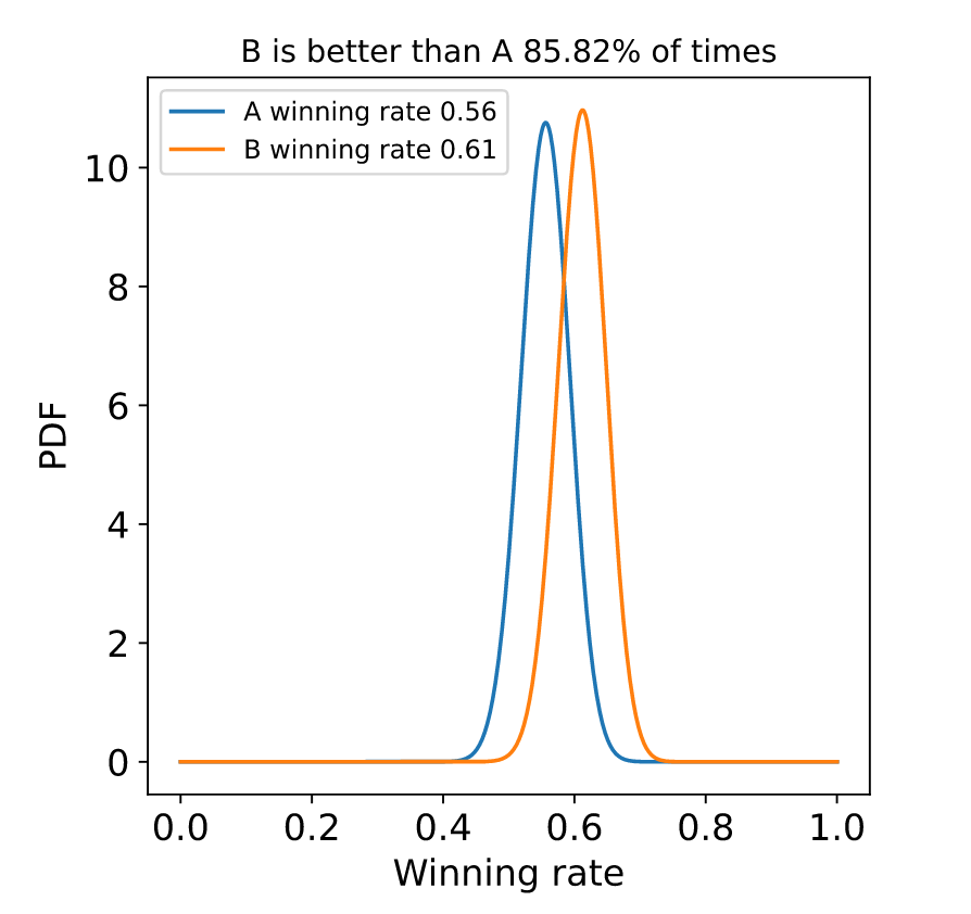
Below you can see the plot of some beta distributions. In the first plot, the parameters are α_A= 100, β_A=80, α_B=110 and β_B=70.
In this second plot, the parameters α_A= 10, β_A=8, α_B=11 and β_B=7.
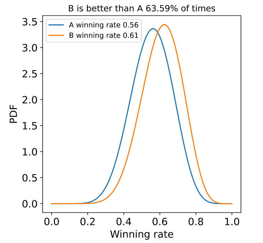
Notice that, even in both cases the winning rates are the same, but the distributions look different. This is because in the first case, we’re more sure about the actual rate, and this is because we’ve observed more points than in the second case.
Family-wise error rate
Usually, in A/B testing one just compares two variations, eg: conversions in a website with white background vs blue background. However, in this experiment, we’re not just comparing two variations, but we’re comparing all the possible pairs of variations -remember that we want to find if there is at least one variation that is better than another variation- therefore, the number of comparisons we are doing is 960*959/2 ~ 5e5. This means that using the typical value of α=0.05 is an error because we need to take into consideration that we’re doing a lot of comparisons. For instance, assuming that the winning probabilities distributions are the same for all the initial positions and using the standard one would have a probability

of at least observing one false positive! This means that even if there’s no statistically significant difference between any pair of variations we’ll still observe at least one false positive. If we want to keep the same α but increase the number of comparisons from 2 to we need then to define an effective α like

and solving

Plugging our values we finally get α_eff =1e-7.
Train/Test split
In the previous sections, we developed the theory to determine if a variation is better than another variation according to the observed data. This is, after having seen some data we build a hypothesis of the form variation B is better than variation A . However, we can’t test the truth of this hypothesis using the same data we used to generate the hypothesis. We need to test the hypothesis against a set of data that we haven’t used yet.
To make this possible we will split the full dataset into two disjoint train and test datasets. The train dataset will be used together with the bayesian A/B testing framework to generate hypotheses of the form B>A. And then, using the test dataset we’ll check if the hypotheses hold.
Notice that this approach makes sense only if the distribution of winning rates doesn’t change over time. This seems a reasonable assumption since, AFAIK, there haven’t been big theoretical advances that have changed the winning probability of certain variations during the last few years. In fact, minimizing the theory and preparation impact on game results is one of the goals of Chess960.
Data preparation
In the previous sections we have implicitly assumed that a game can be either won or lost, however, it can also be drawn. I’ve assigned 1 point for a victory, 1/2 point for a draw, and 0 points for a loss, which is the usual approach in chess games.
Results
In this section, we will apply all the techniques explained above to the lichess dataset. In the dataset, we have more than 13M games, which is ~14K games per variation. However, the dataset contains games for a huge variety of players and time controls (from ELO 900 to 2000, and from blitz to classic games). Therefore, doing the comparisons using all the games would mean ignoring confounder variables. To avoid this problem I’ve only used games for players with an ELO in the range (1800, 2100) and with a blitz time control. I’m aware that these filters do not resemble the reality of top-level contests such as the World Fischer Random Chess Championship, but in lichess data, there are not a lot of classical Chess960 games for high-rated players (>2600), so I will just use the group with more games. After applying these filters we end up with a dataset with ~2.4M games, which is ~2.5K games per variation.
The train/test split has been done using a temporal split. All the games prior to 2022-06-01 are part of the training dataset, and all the games after that date are part of the testing dataset, which accounts for ~80% of the data for training and ~20% for testing.
Generating hypotheses
The first step is to generate a set of hypotheses using A/B testing. The number of variation pairs to compare is pretty big (1e5) and testing all of them would take a lot, so we’ll just compare the 20 variations with the highest winning rates against the 30 variations with the lowest winning rates. This means we’ll have 900 pairs of variations to compare. Here we see the pair of variations with the bigger difference in the train dataset
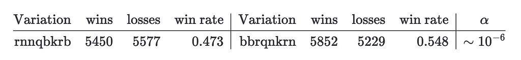
Notice that the α for these variations is bigger than α_eff, which means that the difference is not significant. Since these are the variations with the higher difference we know that there’s not any variation pair with a statistically significant difference.
Anyway, even if the difference is not significant, with this table one can hypothesize that variation rnnqbkrb is worse than variation bbqrnkrn. If we check these variation values in the test dataset we get

Notice that the “bad” variation still has a winning rate lower than the “good” variation, however, it has increased from 0.473 to 0.52, which is quite a lot. This brings a new question: do past variation performance guarantee future performance?
Past vs Future performances
In the last section, we have seen how to generate and test hypotheses, but we have also noticed that the performance of some variations changes over time. In this section, we’ll analyze this question more in detail. To do so, I have computed the winning rate in the train and test datasets and plotted one against the other.
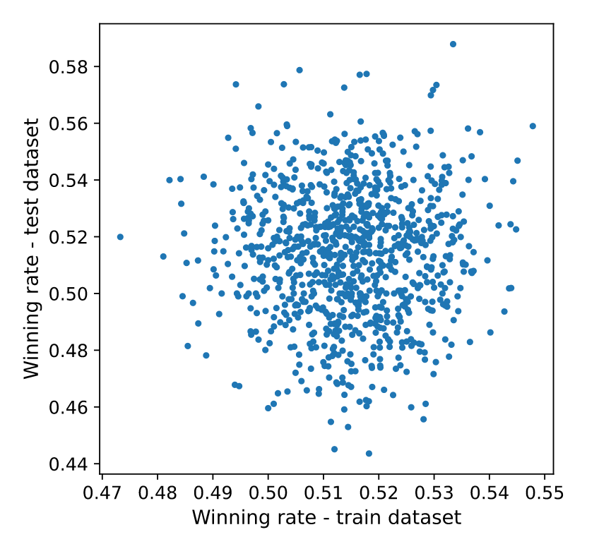
As we can see, there’s no relation between past and future winning rates!
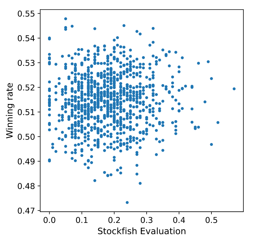
Evaluation vs Rates
We’ve seen that past performances do not guarantee future performances, but do Stockfish evaluations predict future performances? In the following plot, I show the evaluation of Stockfish for each variation and the corresponding winning rate in the dataset.
Machine learning model
Until now we’ve seen that there are no better variations in the Chess960 game and that previous performance is no guarantee of future performance. In this section, we’ll see if we can predict which side is going to win a match based on the variation and the ELO of the players. To do so I’ll train an ML model.
The features of the model are the ELO of the white and black player, the variation being played, and the time control being used. Since the cardinality of the variation feature is huge I’ll use CatBoost, which has been specifically designed to deal with categorical features. Also, as a baseline, I’ll use a model that predicts that white wins if White ELO > Black ELO, draws if White ELO == Black ELO, and losses if White ELO < Black ELO. With this experiment, I want to see which is the impact of the variation in the expected winning rate.
In the next tables, I show the classification reports for both models.
- CatBoost model
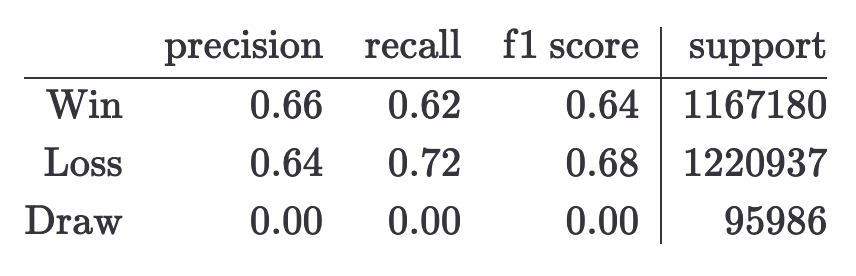
- Baseline model
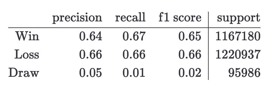
From these tables, we can see that the CatBoost and the baseline model have almost the same results, which means that knowing the variation being played doesn’t help to predict the result of the game. Notice that the results are compatible with the ones obtained here (accuracy ~65%), but in the linked blog it’s assumed that the knowing the variation helps to predict the winner, and we have seen that this is not true.
Conclusions & Comments
In this post, I’ve shown that
- using the standard threshold to determine significant results is not valid when having more than one comparison, and it needs to be adjusted.
- there are no statistically significant differences in the winning rates, ie: we can’t say that a variation is preferable for white than another.
- past rates don’t imply future rates.
- stockfish evaluations don’t predict winning rates.
- knowing which variation is being played doesn’t help to predict the result of a match.
However, I’m aware that the data I’ve used is not representative of the problem I wanted to study in the first place. This is because the data accessible at Lichess is skewed towards non-professional players, and even though I’ve used data from players with a decent ELO (from 1800 to 2100) they are pretty far from the players participating in the Chess960 World Cup (>2600). The problem is that the number of players with an ELO >2600 is very low (209 according to chess.com), and not all of them play regularly Chess960 in Lichess, so the number of games with such characteristics is almost zero.
Analyzing Chess960 Data was originally published in Towards Data Science on Medium, where people are continuing the conversation by highlighting and responding to this story.
...