

 800+ IT
News
als RSS Feed abonnieren
800+ IT
News
als RSS Feed abonnieren📚 A Data-Driven Method to Reduce Employee Survey Length
💡 Newskategorie: AI Nachrichten
🔗 Quelle: towardsdatascience.com
Reducing survey length while maximizing reliability and validity

Employee surveys are quickly becoming a steadfast aspect of organizational life. Indeed, the growth of the people analytics field and the adoption of a data-driven approach to talent management is a testament to this (see McKinsey report). In one survey, we can gather information on how our leaders are performing, whether our workforce is motivated, and if employees are thinking about leaving. There is just one rather long elephant in the room — our survey length.
The creators of employee surveys (e.g., HR and/or behavioral and data scientists) want to measure a multitude of important topics accurately, which often requires a large number of questions. On the other hand, respondents who take long surveys are significantly more likely to dropout from a survey (Hoerger, 2010; Galesic & Bosnjak, 2009) and introduce measurement error (e.g., Peytchev & Peytcheva, 2017; Holtom et al., 2022). Despite this, a greater percentage of respondents are engaging with surveys: published studies in organizational behavior literature have reported a substantial increase in respondent rates from 48% to 68% in a 15-year period (2005–2020; Holtom et al., 2022). While survey length is only one factor amongst a myriad that determine data quality and respondent rates (e.g., incentives, follow-ups; Edwards et al., 2002; Holtom et al., 2022), survey length is easily malleable and under the direct control of survey creators.
This article presents a method to shorten employee surveys by selecting the least amount of items possible to achieve maximal desirable item-level characteristics, reliability, and validity. Through this method, employee surveys can be shortened to save employee time, while hopefully improving participation/dropout rates and measurement error that are common concerns in longer surveys (e.g., Edwards et al., 2002; Holtom et al., 2022; Jeong et al., 2023; Peytchev & Peytcheva, 2017; Porter, 2004; Rolstad et al., 2011; Yammarino et al., 1991).
The Monetary Benefit of Survey Shortening
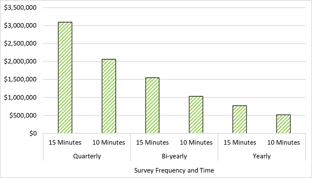
Not convinced? Let’s look at the tangible monetary benefits of shortening a survey. As an illustrative example, let’s calculate the return-on-investment if we shorten a quarterly 15 minute survey to 10 minutes for a large organization of 100,000 individuals (e.g., company in fortune 100). Using the median salary of workers in the United States ($56,287; see report by the U.S. Census), shortening a survey by 5 minutes can save the organization over $1 million in employee time. While these calculations aren’t an exact science, it is a useful metric to understand how survey time can equate into the bottom-line of an organization.
The Solution: Shortening Employee Surveys
To shorten our surveys but retain desirable item-level statistics, reliability, and validity, we leverage a two-step process where Python and R programs will help determine the optimal items to retain. In step 1, we will utilize a multiple-criteria decision making (MCDM) program (Scikit-criteria) to select the best performing items based upon several criteria (standard deviation, skewness, kurtosis, and subject matter expert ratings). In step 2, we will utilize an R program (OASIS; Cortina et al., 2020) to select the optimal combination of top ranked items from step 1 to further shorten our scale but maintain maximal reliability and other validity concerns.
In short, the final output will be a reduced set of items that have desirable item-level statistics and maximal reliability and validity.
Who is this methodology for?
- People analytic professionals, data scientists, I/O psychologists, or human resources (HR) professionals that deal with survey creation and people data
- Ideally, users will have some beginner experience in Python or R and statistics
What do you need?
- Python
- R
- Dataset (Choose one):
- Practice dataset — I utilized the first 1000 responses of a public dataset of the International Personality Item Pool (IPIP; https://ipip.ori.org/; Goldberg, 1992) provided by Open Psychometrics (openpsychometrics.org). For simplicity, I only utilized the 10 conscientiousness items. Note on Data Sources: The IPIP is a public domain personality test that can be utilized without author permission or a fee. Similarly, openpsychometrics.org is open source data that has been utilized in several other academic publications (see here).
- Your own dataset (with responses from employees) for a survey you want to shorten. Ideally, this should be as large of a dataset as possible to improve accuracy and chance of replicability. Generally, most users will want datasets with 100 to 200+ responses to hopefully negate the impact of sampling or skewed responses (see Hinkin, 1998 for further discussion).
- OPTIONAL: Subject Matter Expert (SME) ratings for each item in your dataset that is a candidate for shortening. Only applicable if you are using your own dataset.
- OPTIONAL: Convergent and divergent validity measures. These can be utilized in step two, but is not required. These validity measures are more so important for new scale development rather than shortening an existing established scale. Convergent validity is the degree to which a measure correlates with other similar measures of that construct, whereas divergent validity is the extent to which it is unrelated with non-related measures (Hinkin, 1998; Levy, 2010). Again, only applicable if you have your own dataset.
Github page for code: https://github.com/TrevorCoppins/SurveyReductionCode
Please note: All images, unless otherwise noted, are by the author
Step One: Item-level Analysis and MCDM
Item-level Statistics Explanation
For ‘pure’ item-level statistics (or properties of each item), we utilize standard deviation (i.e., on average, how much do respondents vary in responses) and skewness and kurtosis (i.e., how asymmetrical the distribution of data is and how far it departs from the ideal ‘peakness’ of a normal distribution). A moderate amount of standard deviation is desirable for each item because most of our constructs (e.g., job satisfaction, motivation) naturally differ between individuals. This variability between individuals is what we utilize to make predictions (e.g., “why does the sales department have higher job satisfaction than the research and development department?”). For skewness and kurtosis, we ideally want minimal levels because this indicates our data is normally distributed and is an assumption for a vast majority of our statistical models (e.g., regression). While some skewness and kurtosis are acceptable or even normal dependent on the construct, the real problem arises when distribution of scores has a large difference from a normal distribution (Warner, 2013).
Note: Some variables are not naturally normally distributed and should not be utilized here. For example, frequency data for the question: “In the last month, have you experienced a workplace accident?” is a true non-normal distribution because a vast majority would select ‘None’ (or 0).
Item-level Analysis and MCDM
First, we need to install some programs that are required for later analyses. The first of which is the MCDM program: scikit-criteria (see documentation here; with the Conda install, it may take a minute or two). We also need to import pandas, skcriteria, and the skew and kurtosis modules of scipy.stats.
conda install -c conda-forge scikit-criteria
import pandas as pd
import skcriteria as skc

from scipy.stats import skew
from scipy.stats import kurtosis
Data Input
Next, we need to choose our data: 1) your own dataset or 2) practice dataset (as discussed above, I utilized the first 1000 responses on 10 items of conscientiousness from an open-source dataset of the IPIP-50).
Note: if you are using your own dataset, you will need to clean your data prior to the rest of the analyses (e.g., deal with missing data).
# Data file #

# 1) load your own datafile here
# OR
# 2) Utilize the practice dataset of the first 1000 responses of IPIP-50
# which is available at http://openpsychometrics.org/_rawdata/.
# For simplicity, we only utilized the 10-conscientious items (CSN)

## The original IPIP-50 survey can be found here:
## https://ipip.ori.org/New_IPIP-50-item-scale.htm

Data = pd.read_csv(r'InsertFilePathHere.csv')
If you are using the practice dataset, some items need to be recoded (see here for scoring key). This ensures that all responses are on the same direction for our likert-scale responses (e.g., 5 represents highly conscientious responses across all items).
#Recoding conscientiousness items
Data['CSN2'] = Data['CSN2'].replace({5:1, 4:2, 3:3, 2:4, 1:5})
Data['CSN4'] = Data['CSN4'].replace({5:1, 4:2, 3:3, 2:4, 1:5})
Data['CSN6'] = Data['CSN6'].replace({5:1, 4:2, 3:3, 2:4, 1:5})
Data['CSN8'] = Data['CSN8'].replace({5:1, 4:2, 3:3, 2:4, 1:5})
Note: For this method, you should only work on one measure or ‘scale’ at a time. For example, if you want to shorten your job satisfaction and organizational culture measures, conduct this analysis separately for each measure.
Generating Item-level Statistics
Next, we gather all of the item-level statistics that we need for scikit-criteria to help make our final ranking of optimal items. This includes standard deviation, skewness, and kurtosis. It should be noted that kurtosis program here utilizes Fisher’s Kurtosis, where a normal distribution has 0 kurtosis.
## Standard Deviation ##
std = pd.DataFrame(Data.std())
std = std.T

## Skewness ##
skewdf = pd.DataFrame(skew(Data, axis=0, bias=False, nan_policy='omit'))
skewdf = skewdf.T
skewdf = pd.DataFrame(data=skewdf.values, columns=Data.columns)

## Kurtosis ##
kurtosisdf = pd.DataFrame(kurtosis(Data, axis=0, bias=False, nan_policy='omit'))
kurtosisdf = kurtosisdf.T
kurtosisdf = pd.DataFrame(data=kurtosisdf.values, columns=Data.columns)
OPTIONAL: Subject Matter Expert Ratings (Definitional Correspondence)
While optional, it is highly recommended to gather subject matter expert (SME) ratings if you are establishing a new scale or measure in your academic or applied work. In general, SME ratings help establish content validity or definitional correspondence, which is how well your items correspond to the provided definition (Hinkin & Tracey, 1999). This method involves surveying a few individuals on how closely an item corresponds to a definition you provide on a likert-scale of 1 (Not at all) to 5 (Completely). As outlined in Colquitt et al. (2019), we can even calculate a HTC index with this information: average definitional correspondence rating / number of possible anchors. For example, if 5 SMEs’ mean correspondence rating of item i was 4.20: 4.20/5 = 0.84.
If you have collected SME ratings, you should format and include them here as a separate dataframe. Note: you should format SME ratings into a singular column, with each item listed as a row. This will make it possible to merge the different dataframes.
#SME = pd.read_csv(r'C:\XXX insert own filepath here)
#SME = SME.T
#SME.columns = Data.columns
Merging Data and Absolute Values
Now, we simply merge these disparate data frames of SME (optional) and item-level statistics. The names of the items need to match across dataframes or else pandas will add additional rows. Then, we transpose our data to match our final scikit-criteria program requirements.
mergeddata = pd.concat([std, skewdf, kurtosisdf], axis=0)
mergeddata.index = ['STD', 'Skew', "Kurtosis"]
mergeddata = mergeddata.T
mergeddata
Lastly, since skewness and kurtosis can range from negative to positive values, we take the absolute value because it is easier to work with.
mergeddata['Skew'] = mergeddata['Skew'].abs()
mergeddata['Kurtosis'] = mergeddata['Kurtosis'].abs()
Scikit-criteria Decision-matrix and Ranking Items
Now we utilize the scikit-criteria decision-making program to rank these items based upon multiple criteria. As can be seen below, we must pass the values of our dataframe (mergeddata.values), input objectives for each criteria (e.g., if maximum or minimum is more desirable), and weights. While the default code has equal weights for each criteria, if you utilize SME ratings I would highly suggest assigning more weight to these ratings. Other item-level statistics are only important if we are measuring the construct we intend to measure!
Finally, alternatives and criteria are simply the names passed into the scikit-criteria package to make sense of our output.
dmat = skc.mkdm(
    mergeddata.values, objectives=[max, min, min],
    weights=[.33, .33, .33],
    alternatives=["it1", "it2", "it3", "it4", "it5", "it6", "it7", "it8", "it9", "it10"],
    criteria=["SD", "Skew", "Kurt"])
Filters
One of the greatest parts about scikit-criteria is their filters function. This allows us to filter out undesirable item-level statistics and prevent these items from making it to the final selection ranking stage. For example, we do not want an item reaching the final selection stage if they have extremely high standard deviation — this indicates respondents vary wildly in their answer to questions. For SME ratings (described above as optional), this is especially important. Here, we can only request items to be retained if they score above a minimal threshold — this prevents items that have extremely poor definitional correspondence (e.g., average SME rating of 1 or 2) from being a top ranked item if they have other desirable item-level statistics. Below is an application of filters, but since our data is already within these value limits it does not impact our final result.
from skcriteria.preprocessing import filters

########################### SD FILTER ###########################
# For this, we apply a filter: to only view items with SD higher than .50 and lower than 1.50
# These ranges will shift based upon your likert scale options (e.g., 1-5, 1-7, 1-100)

## SD lower limit filter
SDLL = filters.FilterGE({"SD": 0.50})
SDLL

dmatSDLL = SDLL.transform(dmat)
dmatSDLL

## SD upper limit filter
SDUL = filters.FilterLT({"SD": 1.50})
dmatSDUL = SDUL.transform(dmatSDLL)
dmatSDUL

## Whenever it is your final filter applied, I suggest changing the name
dmatfinal = dmatSDUL
dmatfinal

# Similarly, for SME ratings (if used), we may only want to consider items that have an SME above the median of our scale.
# For example, we may set the filter to only consider items with SME ratings above 3 on a 5-point likert scale

########################### SME FILTER ###########################

# Values are not set to run because we don't have SME ratings
# To utilize this: simply remove the # and change the decision matrix input
# in the below sections

#SMEFILT = filters.FilterGE({"SME": 3.00})

#dmatfinal = SME.transform(dmatSDUL)
#dmatfinal
Note: This can also be applied for skewness and kurtosis values. Many scientists will utilize a general rule-of-thumb where skewness and kurtosis is acceptable between -1.00 and +1.00 (Warner, 2013); you would simply create upper and lower level limit filters as shown above with standard deviation.
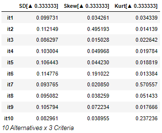
Inversion and Scaling Criteria
Next, we invert our skewness and kurtosis values to make all criteria maximal through invert_objects.InvertMinimize(). The scikit-criteira program prefers all criteria to be maximized as it is easier for the final step (e.g., sum weights). Finally, we scale each criteria for easy comparison and weight summation. Each value is divided by the sum of all criteria in that column to have an easy comparison of optimal value for each criterion (e.g., it1 has an SD of 1.199, which is divided by the column total of 12.031 to obtain .099).
# skcriteria prefers to deal with maxmizing all criteria
# Here, we invert our skewness and kurtosis. Higher values will then be more desirable

from skcriteria.preprocessing import invert_objectives, scalers

inv = invert_objectives.InvertMinimize()
dmatfinal = inv.transform(dmatfinal)

# Now we scale each criteria into an easy to understand 0 to 1 index
# The closer to 1, the more desirable the item statistic

scaler = scalers.SumScaler(target="both")
dmatfinal = scaler.transform(dmatfinal)
dmatfinal
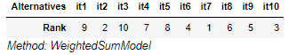
Final Rankings (Sum Weights)
Finally, there are a variety of ways we can use this decision-matrix, but one of the easiest ways is to calculate the weighted sum. Here, each item’s row is summated (e.g., SD + skewness + kurtosis) and then ranked by the program.
## Now we simply rank these items ##

from skcriteria.madm import simple
decision = simple.WeightedSumModel()
ranking = decision.evaluate(dmatfinal)
ranking
For the practice dataset, the rankings are as follows:
Save Data for Step Two
Lastly, we save our original and clean dataset for step two (here, our original ‘Data’ dataframe, not our decision matrix ‘dmatfinal’). In step two, we will input items that have been highly ranked in step one.
## Save this data for step 2 ##

Data.to_csv(r'C:\InputYourDesiredFilePathandName.csv')
Step two: Final Item Optimization for Reliability and Validity
In step one, we ranked all our items according to their item-level statistics. Now, we utilize the Optimization App for Selecting Item Subsets (OASIS) calculator in R, which was developed by Cortina et al. (2020; see user guide). The OASIS calculator runs multiple combinations of our items and determines which combination of items results in the highest level of reliability (and convergent + divergent validity if applicable). For this example, we focus on two common reliability indices: cronbach’s alpha and omega. These indices are typically extremely similar in value, however, many researchers have advocated for omega to be the main reliability indices for a variety of reasons (See Cho & Kim, 2015; McNeish, 2018). Omega is a measure of reliability which determines how well a set of items load onto a singular ‘factor’ (e.g., a construct, such as job satisfaction). Similar to Cronbach's alpha (a measure of internal reliability), higher values are more desirable, where values above .70 (max upper limit = 1.00) are generally considered reliable in academic research.
The OASIS calculator is extremely easy to use due to the shiny app. The following code will install required programs and prompt a pop-up box (as seen below). Now, we select our original cleaned dataset from step one. In our illustrative example, I have selected the top 8 items, requested a minimum of 3 items and a maximum of 8. If you had convergent or divergent validity measures, you can input them in this step. Otherwise, we request for the calculation of omega-h.
install.packages(c("shiny","shinythemes","dplyr","gtools","Lambda4","DT","psych", "GPArotation", "mice"))
library(shiny)
runUrl("https://orgscience.uncc.edu/sites/orgscience.uncc.edu/files/media/OASIS.zip")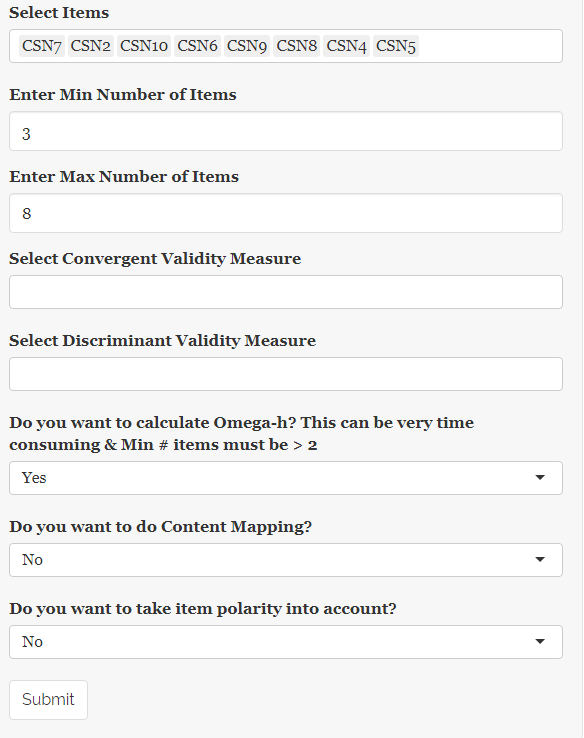
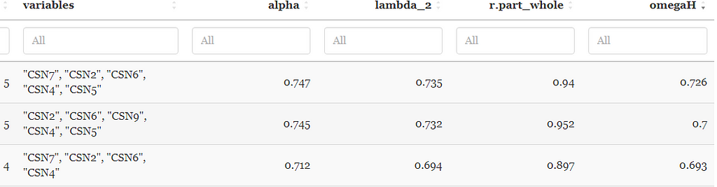
The Final Results
As can be seen below, a 5-item solution produced the highest omega (ω = .73) and Cronbach alpha coefficients (α = .75) which met traditional academic reliability standards. If we had convergent and divergent validity measures, we could also rank item combinations using these values as well. The OASIS calculator also lets you select general ranges for each value (e.g., only show combinations above certain values).
Let’s compare our final solution:
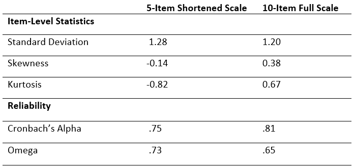
In comparison to the full 10-item measure, our final item set takes half the time to administer, has comparable and acceptable levels of reliability (ω and α >.70), slightly higher standard deviation and lower skewness, but unfortunately higher levels of kurtosis (however, it is still within the acceptable range of -1.00 to +1.00).
This final shortened item-set could be a very suitable candidate to replace the full measure. If successfully replicated for all survey measures, this could substantially reduce survey length in half. Users may want to take additional steps to verify the new shortened measure works as intended (e.g., predictive validity and investigating the nomological network — does the shortened measure have comparable predictions to the full length scale?).
Caveats
- This methodology may produce final results that can be grammatically redundant or lack content coverage. Users should adjust for this by ensuring their final item set chosen in step two has adequate content coverage, or, use the OASIS calculator’s content mapping function (see documentation). For example, you may have a personality or motivation assessment that has multiple ‘subfactors’ (e.g., if you are externally or intrinsically motivated). If you do not content map in OASIS calculator or take this into account, you may end up with only items from one subfactor.
- Your results may slightly change from sample to sample. Since both steps use existing data to ‘maximize’ the outcomes, you may see a slight drop in reliability or item-level statistics in future samples. However, this should not be substantial.
- Dependent on your organization/sample, your data may naturally be skewed because it is from a singular source. For example, if company X requires all managers to engage in certain behaviors, items asking about said behaviors are (hopefully) skewed (i.e., all managers rated high).
Conclusion
This article introduced a two-step method to significantly reduce survey length while maximizing reliability and validity. In the illustrative example with open-source personality data, the survey length was halved but maintained high levels of Cronbach and Omega reliability. While additional steps may be required (e.g., replication and comparison of predictive validity), this method provides users a robust data-driven approach to substantially reduce their employee survey length, which can ultimately improve data quality, respondent dropout, and save employee time.
References
E. Cho and S. Kim, Cronbach’s Coefficient Alpha: Well Known but Poorly Understood (2015), Organizational Research Methods, 18(2), 207–230.
J. Colquitt, T. Sabey, J. Rodell and E. Hill, Content validation guidelines: Evaluation criteria for definitional correspondence and definitional distinctiveness (2019), Journal of Applied Psychology, 104(10), 1243–1265.
J. Cortina, Z. Sheng, S. Keener, K. Keeler, L. Grubb, N. Schmitt, S. Tonidandel, K. Summerville, E. Heggestad and G. Banks, From alpha to omega and beyond! A look at the past, present, and (possible) future of psychometric soundness in the Journal of Applied Psychology (2020), Journal of Applied Psychology, 105(12), 1351–1381.
P. Edwards, I. Roberts, M. Clarke, C. DiGuiseppi, S. Pratap, R. Wentz and I. Kwan, Increasing response rates to postal questionnaires: systematic review (2002), BMJ, 324, 1–9.
M. Galesic and M. Bosnjak, Effects of questionnaire length on participation and indicators of response quality in a web survey (2009), Public Opinion Quarterly, 73(2), 349–360.
L. Goldberg, The development of markers for the Big-Five factor structure (1992), Psychological Assessment, 4, 26–42.
T. Hinkin, A Brief Tutorial on the Development of Measures for Use in Survey Questionnaires (1998), Organizational Research Methods, 1(1), 104–121.
T. Hinkin and J. Tracey, An Analysis of Variance Approach to Content Validation (1999), Organizational Research Methods, 2(2), 175–186.
M. Hoerger, Participant dropout as a function of survey length in Internet-mediated university studies: Implications for study design and voluntary participation in psychological research (2010), Cyberpsychology, Behavior, and Social Networking, 13(6), 697–700.
B. Holtom, Y. Baruch, H. Aguinis and G. Ballinger, Survey response rates: Trends and a validity assessment framework (2022), Human Relations, 75(8), 1560–1584.
D. Jeong, S. Aggarwal, J. Robinson, N. Kumar, A. Spearot and D. Park, Exhaustive or exhausting? Evidence on respondent fatigue in long surveys (2023), Journal of Development Economics, 161, 1–20.
P. Levy, Industrial/organizational psychology: understanding the workplace (3rd ed.) (2010), Worth Publishers.
D. McNeish, Thanks coefficient alpha, we’ll take it from here (2018), Psychological Methods, 23(3), 412–433.
A. Peytchev and E. Peytcheva, Reduction of Measurement Error due to Survey Length: Evaluation of the Split Questionnaire Design Approach (2017), Survey Research Methods, 4(11), 361–368.
S. Porter, Raising Response Rates: What Works? (2004), New Directions for Institutional Research, 5–21.
A. Rolstad and A. Rydén, Increasing Response Rates to Postal Questionnaires: Systematic Review (2002). BMJ, 324.
R. Warner, Applied statistics: from bivariate through multivariate techniques (2nd ed.) (2013), SAGE Publications.
F. Yammarino, S. Skinner and T. Childers, Understanding Mail Survey Response Behavior a Meta-Analysis (1991), Public Opinion Quarterly, 55(4), 613–639.
A Data-Driven Method to Reduce Employee Survey Length was originally published in Towards Data Science on Medium, where people are continuing the conversation by highlighting and responding to this story.
...