

 800+ IT
News
als RSS Feed abonnieren
800+ IT
News
als RSS Feed abonnieren📚 Using Python to Solve One of the Most Common Problems in Engineering
💡 Newskategorie: AI Nachrichten
🔗 Quelle: towardsdatascience.com
Creating a generic framework for operating point analysis

Certain classes of problems come up frequently in engineering. The focus of this article is on a specific type of problem that comes up so often in my daily work that I figured I‘d share how I go about solving it using Python. What type of problem are we talking about? The problem of solving the operating point of a system! Let’s illustrate what I mean with a simple example before diving into something a little more complex with code.
We would like to solve the operating point of the simple circuit shown below. This can be done by rearranging Ohm’s law (V=IR) to isolate the current in terms of the known input voltage and resistance.

Simple, right? Unfortunately, most real world problems are never this easy. For example, what if I told you that as the resistor heats up, it’s resistance value changes, essentially making the resistance a function of current. We end up with an equation of the following form:

Without knowing the actual functional form of the resistance, we can’t just solve for current by isolating it algebraically. Furthermore, what if the equation is complicated and it’s not possible to isolate the current by itself? Or, perhaps the resistance is given in terms of current as tabulated discrete data — then we wouldn’t even have an algebraic expression to manipulate to try to solve for current. How would we go about determining the current in the circuit then? We need a more general approach to solving this problem.
The general solution to a problem like this is to pose it as a root finding problem. This is actually incredibly easy to do — we literally just have to subtract the right hand side of the equation from the left hand side, such that we get an equation that equals zero. Doing so yields the following:

By doing this, we’ve re-posed our problem. Instead of solving for the current directly in terms of all other variables, we can try to find the value of current that can be input into the left hand side of the equation to make it evaluate to zero. Why do we formulate the problem like this? Because there are a ton of numerical algorithms that exist (bisection method, Newton’s method, etc.) to solve this exact kind of problem! And most of the algorithms don’t care how complicated the left hand side of the equation is — it doesn’t even have to have a closed algebraic form (i.e. it could be composed of interpolated discrete data, numerically evaluated integrals, or literally any type of function of arbitrary complexity to evaluate). As long as we can pose our problem in the form of f(x)=0, we can (almost) always find a solution to the problem (and the code can be modified/extended easily if the problem statement changes — no need to re-do algebra).
The rest of this article is going to walk through an example of how to apply the root finding methodology to a slightly more complicated, real-world problem, with emphasis on sound code structuring and organization techniques in Python. Although the problem (determining the flow rate of water in a pipe/pump system) is somewhat domain specific, the methodology and coding techniques that are used are completely general, and applicable to all engineering domains. With this in mind, I will try to keep the physical modeling aspects of the problem to a high level, such that regardless of ones technical background, the primary learning objectives of the article still come through clearly.
As a side note, my domain “specialty” these days lies in the realm of motor controls and power electronics, and I am very far removed from pumping/piping applications. I haven’t touched on the subject in years, but thought it would make for an interesting example of the topic at hand. I’m sure there are plenty of individuals out there that are much more qualified to speak on the specifics of pump/pipe modeling than myself, but my intent with this article is on the methodology — not on how to solve pipe/pump problems. Regardless, I openly welcome comments or suggestions for improvement from those that are more knowledgeable of the field!
The Problem
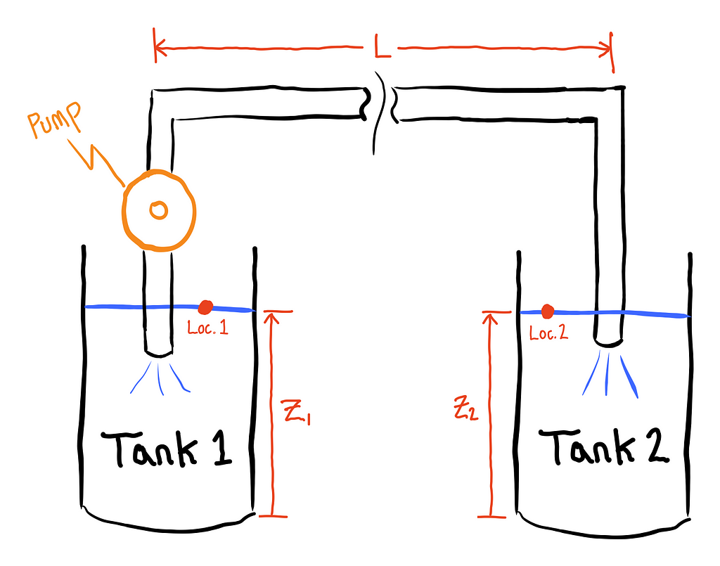
We would like to transfer water from one tank to another. We already have a pump and some piping that can be used to connect the two tanks and want to get an estimate of how long it will take to transfer all of the water. The volume of each tank is known, so if we can estimate the flow rate of water between the tanks, we can estimate how long the transfer process will take. The full apparatus is shown below.
This specific problem (which can be classified as an “internal flow” problem) is very well understood within the field of mechanical engineering. For those less familiar though, or in need of a quick review, the way we typically go about solving these problems is with the Bernoulli equation (shown below).

The Bernoulli equation is essentially an energy conservation statement that tells us how the energy of a fluid particle is transformed between different energy mechanisms as the fluid traverses along a streamline (the flow path that an imaginary particle would follow if dropped in the fluid). The left hand side of the equation represents the total per-weight energy of a fluid particle at any arbitrary first location (location 1) within the fluid, and is the sum of a gravitational potential term, kinetic term, and pressure term. As the fluid traverses the system, energy must be conserved, and thus the total energy at any arbitrary second point (location 2) along the streamline (represented by the right hand side of the equation) must be equal to the total energy at location 1.
The above form of the Bernoulli equation is known as the “head” form of the equation because each term has units of length/height. This is convenient for our intuition because we’re essentially equating the energy of each term to the equivalent gravitational potential energy of a column of fluid with a height of the given head. One major limitation of the Bernoulli equation, however, is that it assumes there are no losses in the system (which isn’t a great assumption). To overcome this limitation, we can supplement the equation with two additional terms as follows:

The Hp(Q) and Hl(Q) terms represent the head added to the system by a pump, and the head lost in the system from real world effects (like friction, viscosity, etc.) respectively. Note that both terms are functions of the system’s fluid flow rate, Q. (As an interesting consequence of the above paragraph describing the interpretation of head, the head of pump tells you how high a pump could theoretically push a fluid). We’ll examine the pump and loss terms more thoroughly in a bit, but before we do, let’s simplify the above equation for our specific problem.
Looking at the system above again, we will conveniently choose our two locations for the Bernoulli equation, such that most of the terms cancel. We can do this by choosing locations 1 and 2 to be at the free surface of the water of each tank respectively, where the pressure is constant and equal to atmospheric pressure (P1=P2), and the velocity is approximately constant and zero (V1=V2=0). We will also assume that the height of the water in the two tanks is the same at the instant we’re analyzing the system such that Z1=Z2. After simplifying the algebra, we see that nearly all of the terms cancel, and we’re left with the fact that the head produced by the pump must equal the head lost in the system due to non-idealities. Stated another way, the pump is making up for any energy losses in the system.

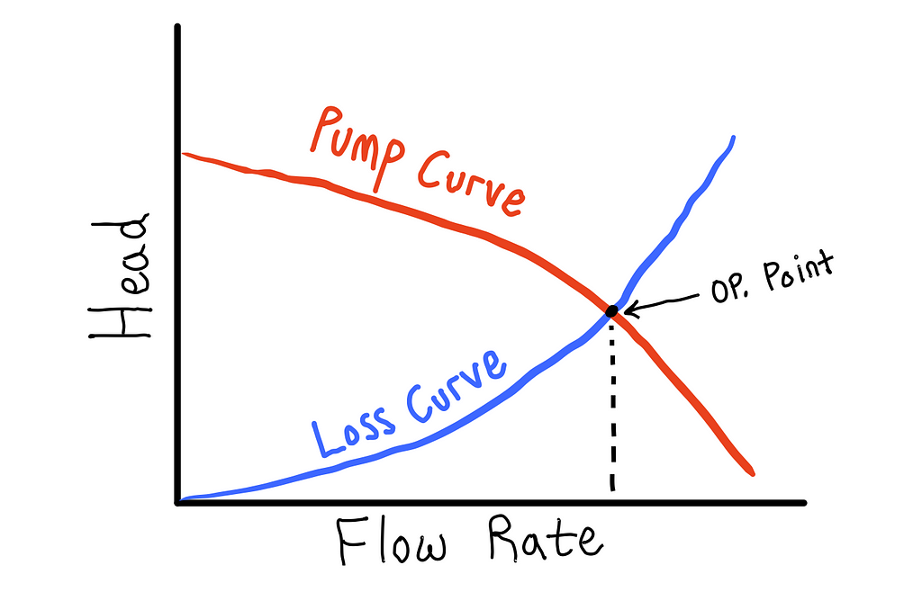
This situation can be seen qualitatively in the figure below. The head produced by a pump decreases with increasing flow rate, whereas, the losses in a piping system increase with increasing flow rate. The point where the two curves intersect (pump head = head loss) determines the operating point (flow rate) of the system.
The last step before we can jump into code is to pose the problem as a root finding problem. Subtracting the right hand side of the equation from the left hand side, we obtain the root solving problem that we are looking for. That is, we’ve posed our problem as follows: find the flow rate (Q) such that the left hand side of the equation below equals zero. At this point, the pump head will equal the system head losses.

The Code
To avoid losing the big picture of what we’re doing, I’m not going to explain every little detail of the code (I’m assuming you have a reasonable background in Python already). Instead, I’m going to focus my efforts on ensuring the narrative and structuring of the code is clear, and go into more detail as needed. As always, feel free to ask any questions if something isn’t clear.
Setup
We will begin by importing all of the necessary modules. It will become apparent how each of the modules is used later on, but it’s worth noting that the key import statements are the ones from scipy. These are the functions that are specific to the problem at hand. The code block also set’s some default plotting settings (to personal taste), creates a folder to save the generated figures in, and defines some unit conversion constants that make our life easier later in the code.
from dataclasses import dataclass
from pathlib import Path

import numpy as np
import matplotlib.pyplot as plt
import pandas as pd

#these are the key libraries for solving the problem
from scipy.interpolate import interp1d
from scipy.optimize import root_scalar

#set plotting defaults
plt.style.use('seaborn-v0_8-darkgrid')
plt.rcParams['font.family'] = 'Times New Roman'
plt.rcParams['font.size'] = 12
figsize = (6.4,4)

#make folder to save plots to
plots_folder = Path('plots')
plots_folder.mkdir(exist_ok=True)

#define conversion constants for ease of use later
INCHES_TO_METERS = 25.4/1000
FEET_TO_METERS = 12*INCHES_TO_METERS
GALLONS_TO_M3 = 0.0037854118 #convert gallons to m^3
Next we will make a Python dataclass that essentially acts as a container for storing fluid properties (density, viscosity, and gravity). By default the properties are set to those of water. Note that although not completely necessary, Python data classes are incredibly convenient. If they’re new to you, I highly recommend you check out this video.
@dataclass
class Fluid():
    #fluid defaults to water properties
    rho: float = 997 #kg/m^3
    mu: float = 0.0007972 #N-s/m^2 = kg/m-s
    g: float = 9.81 #m/s^2
Pipe Model
The next step is to model the head losses of the pipe (the Hl(Q) term in the extended Bernoulli equation above). This is typically done using the Darcy-Weisbach equation shown below, where f is a friction factor (more on this shortly), v is the flow velocity, g is gravity, and L and D are the pipe length and diameter respectively.

Unfortunately, the friction factor (f) isn’t constant, but also depends on the flow velocity, fluid properties, and pipe dimensions. Various models exist to compute f, but we will use Haaland’s equation, shown below.

In this equation, epsilon is the surface roughness of the pipe (which can be found in engineering textbook tables), and Re is the famous Reynolds number, computed as per below.

Lastly, we can note that the swept volume per unit time, or volumetric flow rate (Q) equals the cross-sectional area (A) of the pipe times the flow velocity (v). Thus, given a flow rate in the pipe, we can compute the corresponding flow velocity in the pipe as:

Hopefully all of these equations aren’t detracting from the bigger picture— we’re just looking at one particular model of computing head loss in a pipe. Given a flow rate and pipe dimensions, first compute the corresponding flow velocity, then plug through the equations above to compute the pipe’s head loss. This is exactly what the Pipe class (shown below) implements.
The initialization method stores the pipes dimensions (all assumed to be in meters) and fluid properties. The A method computes the cross-sectional area of the pipe (for those unfamiliar with the@property decorator, this article explains it very well). The Q_to_v method converts the flow rate in gallons per minute (gpm) to a flow velocity in m/s. The friction_factor method evaluates Haaland’s equation as described above, and the head_loss and head_loss_feet evaluate the pipe’s head loss in meters and feet respectively (using the Darcy-Weisbach equation).
class Pipe():

    def __init__(self, L, D, epsilon, fluid: Fluid):

        #pipe dimensions are all assumed to be in meters
        self.L = L
        self.D = D
        self.epsilon= epsilon

        #fluid properties
        self.fluid = fluid

    @property
    def A(self):
        """computes cross-sectional area of pipe in m^2"""

        return np.pi*(self.D/2)**2 #area in m^2

    def Q_to_v(self, gpm):
        """Converts gpm to fluid speed in pipe in m/s"""

        Q = gpm*GALLONS_TO_M3/60 #flow rate in m^3/s
        return  Q/self.A #flow velocity in m/s

    def friction_factor(self, gpm):
        """computes Darcy friction factor, given flow rate in gpm

        This method uses Haaland's equation, wich is an explicit approximation
        of the well-known, but implicit Colebrook equation
        """
        #first get flow velocity from flow rate and pipe dimensions
        v = self.Q_to_v(gpm)
        #compute Reynold's number
        Re = self.fluid.rho*v*self.D/self.fluid.mu
        #compute relative roughness
        e_over_d = self.epsilon/self.D
        #use Haaland's equation
        f = (-1.8*np.log10((e_over_d/3.7)**1.11 + 6.9/Re))**-2
        return f

    def head_loss(self, gpm):
        """computes head loss in meters, given flow rate in gpm"""

        #get flow velocity
        v = self.Q_to_v(gpm)
        #get Darcy friction factor
        f = self.friction_factor(gpm)
        #compute head loss in meters
        hl = 0.5*f*(self.L/self.D)*v**2/self.fluid.g
        return hl

    def head_loss_feet(self, gpm):
        """computes head loss in feet, given flow rate in gpm"""

        hl_meters = self.head_loss(gpm)
        return hl_meters/FEET_TO_METERS
Let’s see the pipe class in action. First, we can create a Fluid object for water and a Pipe object that’s 100 feet long and 1.25 inches in diameter.
#create fluid object for water
water = Fluid()

#create pipe segment with water flowing in it
pipe = Pipe(L=100*FEET_TO_METERS,
            D=1.25*INCHES_TO_METERS,
            epsilon=0.00006*INCHES_TO_METERS,
            fluid=water)
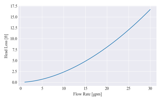
Next we’ll plot the head loss curve as a function of the flow rate in gpm. Isn’t it incredible how clean and easy the code below becomes when we exploit object oriented programming?
gpm_arr = np.linspace(1,30,100)
hl = [pipe.head_loss_feet(gpm) for gpm in gpm_arr]

fig, ax = plt.subplots(figsize=figsize)
ax.plot(gpm_arr, hl)
ax.set_xlabel('Flow Rate [gpm]')
ax.set_ylabel('Head Loss [ft]')
fig.tight_layout()
fig.savefig(plots_folder/'pipe_loss_curve.png')
Pump Model
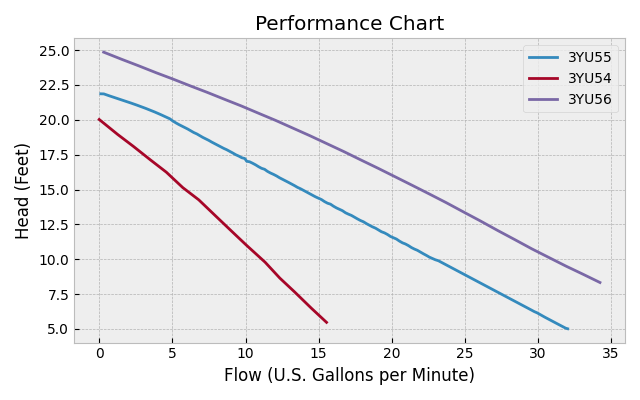
We’ve got a working model of the pipe head losses — now we need a model of the head produced by a pump, Hp(Q). I’m sure there are analytic models that can be used to determine a pumps behavior, but we will assume that we already have a specific pump — namely the following random, fractional horspower pump that I found online:
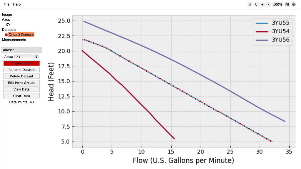
Most pumps will have a data sheet that includes a corresponding pump curve that characterizes the pumps behavior. For our pump, we get the pump curve below (note that for copyright reasons, this is a recreation of the figure provided by the manufacturer — the original can be found here).
At this point we have an image depicting the pumps behavior, but not a mathematical model that can actually be used to determine how it will perform in the system. This issue comes up all the time, and the way I get around it is to 1) digitize the data, and then 2) wrap the discrete data with an interpolation scheme to produce a continous function. Let me illustrate.
Step 1) There are many tools that exist to digitize image data — my personal favorite is the free online utilitiy WebPlotDigitizer. You load in the plot image of interest, align the axes, and then extract the desired data curves (either manually, or with the automatic extraction tool). The data can then be exported to a .csv file.
Step 2) Now that we’ve got digitized data, we just need to wrap it with some sort of interpolator — this is exactly what the Pipe class does below. The initialization method takes in the .csv file name, stores the file name, loads the data into a pandas DataFrame, storing it in a data attribute, and then passes the data to the interp1d function from scipy. The interp1d function then generates a new function that, by default, uses linear interpolation to turn the discrete datapoints into a continous function (full documentation for interp1d function can be found here). The newly generated interpolation function is then stored in a _interp attribute for later access. The Pipe class also contains a bounds method that returns a list containing the min/max values of flow rate in the pump curve data (this will be used in the root finding algorithm), and a head_gain_feet method that takes in the flow rate in gpm, and calls the underlying interpolation function that was generated by interp1d.
class Pump():

    def __init__(self, file):
        #store file name
        self.file = file
        #read data into pandas dataframe and assign column names
        self.data = pd.read_csv(file, names=['gpm', 'head [ft]']).set_index('gpm')
        #create continuous interpolation function
        self._interp = interp1d(self.data.index.to_numpy(), self.data['head [ft]'].to_numpy())

    @property
    def bounds(self):
        """returns min and max flow rates in pump curve data"""
        return [self.data.index.min(), self.data.index.max()]

    def head_gain_feet(self, gpm):
        """return head (in feet) produced by the pump at a given flow rate"""
        return self._interp(gpm)
We can create a Pump object and look at the raw data that we’ve read in.
pump = Pump('pump_data.csv')
pump.data.head()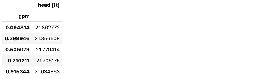
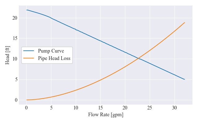
We can also plot the pump curve data with the pipe loss curve to visually see where the system will operate.
head_loss = [pipe.head_loss_feet(gpm) for gpm in pump.data.index]

fig, ax = plt.subplots(figsize=figsize)
ax.plot(pump.data, label='Pump Curve')
ax.plot(pump.data.index, head_loss, label='Pipe Head Loss')
ax.set_xlabel("Flow Rate [gpm]")
ax.set_ylabel("Head [ft]")
ax.legend(frameon=True, facecolor='w', framealpha=1, loc=6)
fig.tight_layout()
fig.savefig(plots_folder/'pump_curve_with_losses.png')
System Model
We finally have the infrastructure in place to solve the operating point of the pump/pipe system. The last step is to create a System class that takes in a Pipe and Pump object and performs the root solving operation. As can be seen in the code below, the System class takes in and stores a Pipe and Pump object. It then uses the two objects to create a residual method that computes the difference between the pump head and pipe head loss. This residual method is then used in theget_operating_point method to actually solve the operating point of the system. The method wraps the root_scalar function from scipy, which acts as an interface for various root solving algorithms. We will let the root_scalar function choose whichever algorithm it sees best fit, but to help it, we will specify a bracketing interval that we know the root lies between. In our case, this bracketing interval is the upper and lower flow-rate bounds of the pump curve data. Full documentation on the root_scalar function can be found here.
Pro tip: the process of injecting the Pipe and Pump objects into the System class (as opposed to having the system class create a Pipe and Pump object at instantiation) is called “dependency injection”. This is typically considered a good coding practice as it makes code more modular, extensible, and easier to debug/test.
class System():

    def __init__(self, pipe: Pipe, pump: Pump):
        self.pipe = pipe
        self.pump = pump

    def residual(self, gpm):
        """
        Computes the difference between the head produced by the pump
        and the head loss in the pipe. At steady state, the pump head and
        head loss will be equal and thus the residual function will go to zero
        """
        return self.pump.head_gain_feet(gpm) - self.pipe.head_loss_feet(gpm)

    def get_operating_point(self):
        """solve for the flow rate where the residual function equals zero.
        i.e. the pump head equals the pipe head loss"""
        return root_scalar(sys.residual, bracket=pump.bounds)
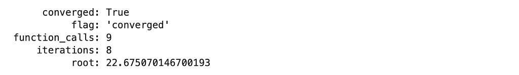
Let’s create a System and run the get_operating_point method to observe the fruits of our labor. As can be seen by the code output, the get_operating point method simply passes out the output of the root_scalar function, which is a RootResults object. This object is essentially just a container that stores various attributes, the most important of which, is the root attribute as it contains the solution to our problem.
sys = System(pipe, pump)

res = sys.get_operating_point()
res
We can plot the same pump and head loss curves again, this time adding in a vertical line at the computed steady-state operating point.
head_loss = [pipe.head_loss_feet(gpm) for gpm in pump.data.index]

fig, ax = plt.subplots(figsize=figsize)
ax.plot(pump.data, label='Pump Curve')
ax.plot(pump.data.index, head_loss, label='Pipe Head Loss')
#plot vertical line at operating point
ax.axvline(res.root, color='k', ls='--', lw=1)
ax.legend(frameon=True, facecolor='white', framealpha=1, loc=6)
ax.set_xlabel("Flow Rate [gpm]")
ax.set_ylabel("Head [ft]")
ax.set_title(f'Operating Point = {res.root:.1f} gpm')
fig.tight_layout()
fig.savefig(plots_folder/'intersection_solution.png')
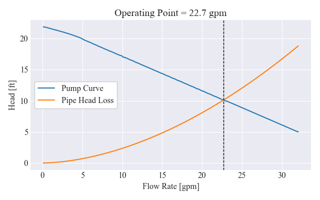
Voila! We’ve programmatically determined the operating point of our system. And because we’ve done it using a somewhat generic coding framework, we can easily try the same analysis using different pumps or piping! We could even extend our code to include multiple pumps, or various pipe fittings/pipe branches.
Design Exploration
As a final little example, highlighting the benefits of setting up the code the way we did, we will perform a design exploration. Using the same pump, we would like to understand the impacts that pipe length has on the volumetric flow rate in the system. To do this, we simply loop over an array of pipe lengths (ranging from 100 to 1000 feet), update the length attribute of the Pipe object stored in the System, and then re-compute the operating point of the system, appending the result to a list. Finally we plot water flow rate as a function of pipe length.
#sweep pipe length from 100 to 1000 feet
lengths_feet = np.linspace(100, 1000, 1000)
lengths_meters = lengths_feet*FEET_TO_METERS

flow_rates = []
for l in lengths_meters:
    #update pipe length
    sys.pipe.L = l
    #compute new flow rate solution
    res = sys.get_operating_point()
    #append solution to flow rates list
    flow_rates.append(res.root)

#plot results
fig, ax = plt.subplots(figsize=figsize)
ax.plot(lengths_feet, flow_rates)
ax.set_xlabel("Pipe Length [ft]")
ax.set_ylabel("Flow Rate [gpm]")
# ax.set_ylim(bottom=0)
fig.tight_layout()
fig.savefig(plots_folder/'flow_vs_pipe_length.png')
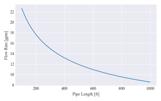
In a few lines of code, we were able to extract meaningful insight into the behavior of our system. If this was a design problem, these insights could drive key design choices.
Conclusion
This article, although focused strongly on a domain specific example problem, highlights a few aspects of a work flow that I end up using a lot. The problem of operating point analysis comes up constantly in engineering and science, and although there are many ways to approach the issue, some methods are more robust, extensible, and flexible than others. The methodology (problem formulation and code structuring principles) used in this article have served me incredibly well, and I hope that others are inspired to adopt a similar work flow!
Feel free to leave any comments or questions you may have or connect with me on Linkedin — I’d be more than happy to clarify any points of uncertainty. Finally, I encourage you to play around with the code yourself (or even use it as a starting template for your own workflows ) — the Jupyter Notebook for this article can be found on my Github.
Nicholas Hemenway
- If you enjoyed this, please follow me on Medium
- Consider subscribing to email updates
- Interested in collaborating? Let’s connect on LinkedIn
Using Python to Solve One of the Most Common Problems in Engineering was originally published in Towards Data Science on Medium, where people are continuing the conversation by highlighting and responding to this story.
...