

 800+ IT
News
als RSS Feed abonnieren
800+ IT
News
als RSS Feed abonnieren📚 An Intuitive Explanation for Inverse Propensity Weighting in Causal Inference
💡 Newskategorie: AI Nachrichten
🔗 Quelle: towardsdatascience.com
Understanding the roots of inverse propensity weighting through a simple example.

One of the well-established methods for causal inference is based on the Inverse Propensity Weighting (IPW). In this post we will use a simple example to build an intuition for IPW. Specifically, we will see how IPW is derived from a simple weighted average in order to account for varying treatment assignment rates in causal evaluation.
Let’s consider the simple example where we want to estimate the average effect of running a marketing coupon campaign on customer spending. We run the campaign in two stores by randomly assigning a coupon to existing customers. Suppose both stores have same number of customers and, unknown to us, spending among treated customers is distributed as N(20,3²) and N(40,3²) in stores 1 and 2, respectively.
Throughout the example Yi(1) represents an individual’s spending if they receive a coupon, Ti=1, and Yi(0) represents their spending if they don’t, Ti=0. These random variables are called potential outcomes. The observed outcome Yi is related to potential outcomes as follows:
https://medium.com/media/79b8e7da12868fe09672c134c5aa4c40/hrefOur estimand, the thing that we want to estimate, is the population mean spending given a coupon, E[Yi(1)]. If we randomly assign coupons to the same number of customers in both stores, we can get an unbiased estimate of this by simply averaging the observed spending of the treated customers, which is 0.5∗$20+0.5∗$40=$30.
Mathematically, this looks as follows:
https://medium.com/media/16d712ca4d14c98b5e552131947c9144/hrefwhere the first equation is due to the potential outcomes, and the last equation follows from random assignment of treatment, which makes potential outcomes independent of treatment assignment:
https://medium.com/media/fcbb9bc6f30b58d115454fec0c14b574/hrefSimple Average
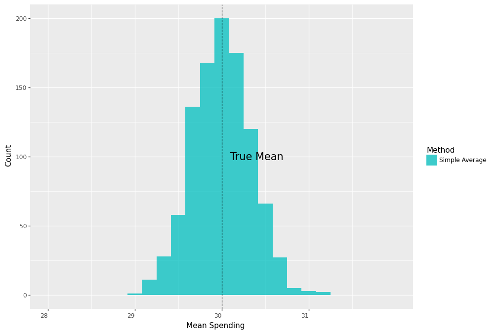
Let’s define a function that generates a sample of 2000 customers, randomly assigns 50% of them to treatment in both stores, and records their average spending. Let’s also run a simulation that calls this function for 1000 times.
def run_campaign(biased=False):
    true_mu1treated , true_mu2treated = 20 , 40
    n, p , obs = 1, .5 , 2000 # number of trials, probability of each trial,
                              # number of observations
    store = np.random.binomial(n, p, obs)+1
    df = pd.DataFrame({'store':store})
    probtreat1 = .5

    if biased:
        probtreat2 = .9
    else:
        probtreat2 = .5

    treat = lambda x: int(np.random.binomial(1, probtreat1, 1))\
                   if x==1 else int(np.random.binomial(1, probtreat2, 1))

    spend = lambda x: float(np.random.normal(true_mu1treated, 3,1))\
                   if (x[0]==1 and x[1]==1)\
                   else ( float(np.random.normal(true_mu2treated, 3,1) ) )

    df['treated'] = df['store'].apply(treat)
    df['spend'] = df[['store','treated']].apply(tuple,1).apply(spend)

    simple_value_treated = np.mean(df.query('treated==1')['spend'])

    return [simple_value_treated]
sim = 1000
values = Parallel(n_jobs=4)(delayed(run_campaign)() for _ in tqdm(range(sim)))
results_df = pd.DataFrame(values, columns=['simple_treat'])
The following plot shows that the distribution of the average spending is centered around the true mean.
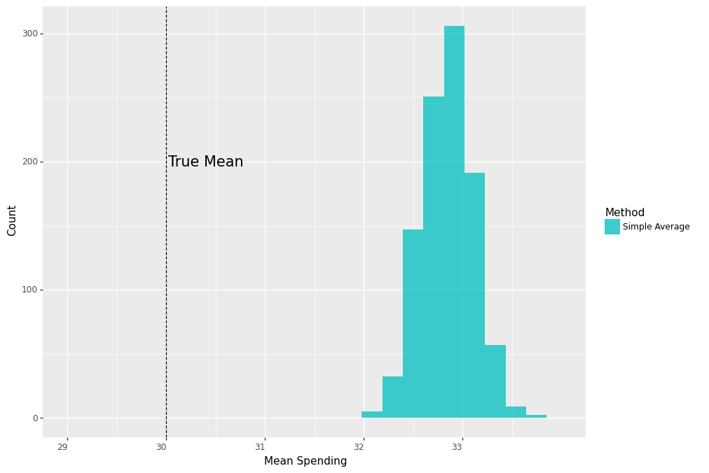
Now, suppose for some reason the second store assigned coupons to 90% of the customers, whereas the first store assigned it to 50%. What happens if we ignore this and use the same approach as previously and take an average of all treated customers’ spending? Because customers of the second store have a higher treatment rate, their average spending will take a larger weight in our estimate and thereby result in an upward bias.
In other words, we no longer have a truly randomized experiment because the probability of receiving a coupon now depends on the store. Moreover, because treated customers in the two stores also have substantially different spending on average, the store a customer belongs to is a confounding variable in causal inference speak.
Mathematically, if we use the simple average spending of treated customers, this time, instead of having this:
https://medium.com/media/4c28e4d1ad0d863762a1c1b227419998/hrefwe end up with this:
https://medium.com/media/882b0860aec142b0ea2da6776290535b/hrefIndeed, repeating the simulation and plotting the results, we see that the distribution of the average spending is now centered far from the true mean.
sim = 1000
values = Parallel(n_jobs=4)(delayed(run_campaign)(biased=True) for _ in tqdm(range(sim)) )
results_df = pd.DataFrame(values, columns=['simple_treat'])
Weighted Average
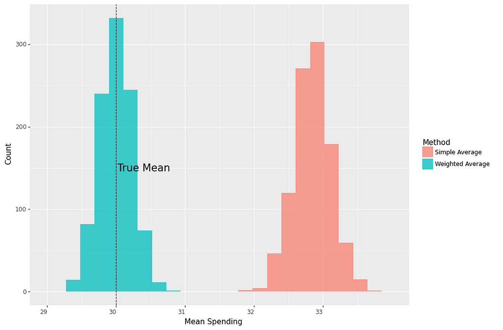
All is not lost, however. Since we know that our experiment was messed up because assignment rates were different between stores, we can correct it by taking a weighted average of treated customers’ spending, where weights represent the proportion of customers in each store. This means, we can reclaim random assignment of treatment once we condition on the store information:
https://medium.com/media/c68ff829d5bcf9cb371d34ed5cb613a9/hrefwhere Xi represents store membership of customer i
https://medium.com/media/12b13005f886a287150fd47482cd3cb5/hrefand obtain unbiased estimates of our causal estimand, E[Yi(1)].
The math now works as follows:
https://medium.com/media/12e597d15a721c28fe342a66fdbbf3d1/hrefwhere the first equation is due to the law of iterated expectations and the second one is due to conditional independence.
Let n1 and n2 denote the number of customers in both stores. Similarly, let n1T and n2T represent the number of treated customers in both stores. Then the above estimator can be computed from the data as follows:
https://medium.com/media/f18b257c073164505179733af7e5d51c/hrefSure enough, if we repeat the previous sampling process
def run_campaign2():
    true_mu1treated , true_mu2treated = 20, 40
    n, p , obs = 1, .5 , 2000 # number of trials, probability of each trial,
                              # number of observations
    store = np.random.binomial(n, p, obs)+1
    df = pd.DataFrame({'store':store})

    probtreat1 = .5
    probtreat2 = .9

    treat = lambda x: int(np.random.binomial(1, probtreat1, 1))
                   if x==1 else int(np.random.binomial(1, probtreat2, 1))

    spend = lambda x: float(np.random.normal(true_mu1treated, 3, 1))
                   if (x[0]==1 and x[1]==1)
                   else ( float(np.random.normal(true_mu2treated, 3, 1) ) )

    df['treated'] = df['store'].apply(treat)
    df['spend'] = df[['store','treated']].apply(tuple,1).apply(spend)

    simple_value_treated = np.mean(df.query('treated==1')['spend'])

    prob1 = df.query('store==1').shape[0]/df.shape[0]
    prob2 = df.query('store==2').shape[0]/df.shape[0]

    est_mu1treated = np.mean(df.query('treated==1 & store==1')['spend'])
    est_mu2treated = np.mean(df.query('treated==1 & store==2')['spend'])

    weighted_value_treated = prob1*est_mu1treated + prob2*est_mu2treated

    return [simple_value_treated, weighted_value_treated]
sim = 1000
values = Parallel(n_jobs=4)(delayed(run_campaign2)() for _ in tqdm(range(sim)) )
results_df = pd.DataFrame(values, columns=['simple_treat','weighted_treat'])
we see that the average of weighted averages is again right on the true mean.
IPW
Let’s now do some algebraic manipulation by rewriting the mean spending in store 1:
https://medium.com/media/8242b02980eadddb3a3ff089632b5954/hrefDoing the same for store 2 and plugging them back in we have the following:
https://medium.com/media/176b6bc03ee74123914dafa7d98d3fba/hrefDenote the proportion of treated customers in store 1 as
https://medium.com/media/6c6df1be7236b5227f9a6c7cf6f81ff5/hrefand similarly for store 2, then we can simplify the previous equation into:
https://medium.com/media/944b3e52347f4694990534c5f53593fa/hrefwhere p(Xi) is the probability of receiving treatment conditional on the confounding variable, aka the propensity score,
https://medium.com/media/7b10a7fbdb3f95d7e8981426584449da/hrefNotice, we started with one weighted average and ended up with just another weighted average that uses
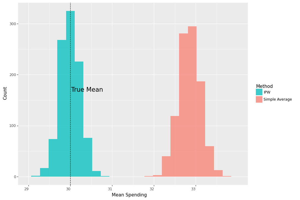
https://medium.com/media/7f31ca449e637c30ce9efa1355e29563/hrefas weights. This is the well-known inverse propensity weighted estimator.
Running the previous analysis with this estimator
def run_campaign3():
    true_mu1treated , true_mu2treated = 20, 40
    n, p , obs = 1, .5 , 2000 # number of trials, probability of each trial,
                              # number of observations
    store = np.random.binomial(n, p, obs)+1
    df = pd.DataFrame({'store':store})

    probtreat1 = .5
    probtreat2 = .9

    treat = lambda x: int(np.random.binomial(1, probtreat1, 1))
                   if x==1 else int(np.random.binomial(1, probtreat2, 1))

    spend = lambda x: float(np.random.normal(true_mu1treated, 3, 1))
                   if (x[0]==1 and x[1]==1)
                   else ( float(np.random.normal(true_mu2treated, 3, 1) ) )

    df['treated'] = df['store'].apply(treat)
    df['spend'] = df[['store','treated']].apply(tuple,1).apply(spend)

    prob1 = df.query('store==1').shape[0]/df.shape[0]
    prob2 = df.query('store==2').shape[0]/df.shape[0]

    simple_value_treated = np.mean(df.query('treated==1')['spend'])

    #estimate propensity score:
    ps1 = df.query('treated==1 & store==1').shape[0]/df.query('store==1').shape[0]
    ps2 = df.query('treated==1 & store==2').shape[0]/df.query('store==2').shape[0]
    df['ps'] = pd.Series(np.where(df['store']==1, ps1, ps2))
    ipw_value_treated = np.mean( (df['spend']*df['treated'])/df['ps'])

    return [simple_value_treated, ipw_value_treated]
sim=1000
values = Parallel(n_jobs=4)(delayed(run_campaign3)() for _ in tqdm(range(sim)) )
results_df = pd.DataFrame(values, columns=['simple_treat','ipw_treat'])
gives us the same unbiased estimate as before.
Estimating the Average Treatment Effect
Now, our ultimate goal is to learn the average incremental spending that the marketing campaign has generated, aka the average treatment effect. To do that we need to also estimate the the population mean spending not given a coupon, E[Y_i(0)] and compare it against E[Y_i(1)]. Our estimand is now this:
https://medium.com/media/2af8af50de35479df1c2d95abb6798bf/hrefTowards this, first we repeat the same argument for non-treated and obtain an unbiased estimate for E[Y_i(0)] as follows:
https://medium.com/media/43f46460f45ae4b98f10966a37e959b8/hrefand finally combine them into estimating the impact:
https://medium.com/media/236cc5f8ef6a7ae830c206c7aba6cea5/hrefLet’s now extend our previous analysis into estimating the impact of the campaign. Suppose spending among non-treated customers is distributed as N(10,2²) in both stores, so that the true effect of the campaign is 0.5*$10 + 0.5*$30 = $20.
def run_campaign4():
    true_mu1treated , true_mu2treated = 20, 40
    true_mu1control , true_mu2control = 10, 10
    n, p , obs = 1, .5 , 2000 # number of trials, probability of each trial, number of observations
    store = np.random.binomial(n, p, obs)+1
    df = pd.DataFrame({'store':store})

    probtreat1 = .5
    probtreat2 = .9

    treat = lambda x: int(np.random.binomial(1, probtreat1, 1))
                   if x==1 else int(np.random.binomial(1, probtreat2, 1))

    spend = lambda x: float(np.random.normal(true_mu1treated, 3, 1))
                   if (x[0]==1 and x[1]==1)
                   else ( float(np.random.normal(true_mu2treated, 3, 1) )
                   if  (x[0]==2 and x[1]==1)
                                                                                              else (float(np.random.normal(true_mu1control, 2, 1) ) if  (x[0]==1 and x[1]==0)
                                                                                    else  float(np.random.normal(true_mu2control, 2, 1))     )
    df['treated'] = df['store'].apply(treat)
    df['spend'] = df[['store','treated']].apply(tuple,1).apply(spend)

    prob1 = df.query('store==1').shape[0]/df.shape[0]
    prob2 = df.query('store==2').shape[0]/df.shape[0]

    simple_value_treated = np.mean(df.query('treated==1')['spend'])
    simple_value_control = np.mean(df.query('treated==0')['spend'])

    simple_tau = simple_value_treated - simple_value_control

    est_mu1treated = np.mean(df.query('treated==1 & store==1')['spend'])
    est_mu2treated = np.mean(df.query('treated==1 & store==2')['spend'])

    weighted_value_treated = prob1*est_mu1treated + prob2*est_mu2treated

    est_mu1control = np.mean(df.query('treated==0 & store==1')['spend'])
    est_mu2control = np.mean(df.query('treated==0 & store==2')['spend'])

    weighted_value_control = prob1*est_mu1control + prob2*est_mu2control
    weighted_tau = weighted_value_treated - weighted_value_control

    #estimate propensity score:
    ps1 = df.query('treated==1 & store==1').shape[0]/df.query('store==1').shape[0]
    ps2 = df.query('treated==1 & store==2').shape[0]/df.query('store==2').shape[0]

    df['ps'] = pd.Series(np.where(df['store']==1, ps1, ps2))

    ipw_value_treated = np.mean( (df['spend']*df['treated'])/df['ps'])
    ipw_value_control = np.mean( (df['spend']*(1-df['treated']) )/(1-df['ps'] ))
    ipw_tau = ipw_value_treated - ipw_value_control

    return [simple_tau, weighted_tau, ipw_tau]
sim=1000
values = Parallel(n_jobs=4)(delayed(run_campaign4)() for _ in tqdm(range(sim)) )
results_df = pd.DataFrame(values, columns=['simple_tau','weighted_tau','ipw_tau'])
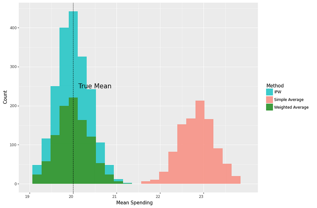
As shown below, both the weighted average and the IPW estimator are centered around the true effect of $20, whereas the distribution of the simple average without controlling for store membership is centered around $23, 15% larger than the true effect.
Conclusion
The IPW estimator has a long history in causal inference. The goal of this post was to develop an intuition for this well-known estimator through a simple example. Using a marketing case we have seen that the hallmark of this method is to correct for unequal treatment assignment mechanisms. Moreover, we have shown that the method is an extension of the weighted average estimator.
References
[1] Richard K. Crump, V. Joseph Hotz, Guido W. Imbens, Oscar A. Mitnik. Dealing with limited overlap in estimation of average treatment effects. (2009), Biometrika.
[2] Stefan Wager, Stats 361: Causal Inference (Spring 2020), Stanford University.
Code
The code for this analysis can be found in my github repository.
Thanks for reading!
My goal is to record my own learning and share it with others who might find it useful. Please let me know if you find any mistakes or have any comments/suggestions.
An Intuitive Explanation for Inverse Propensity Weighting in Causal Inference was originally published in Towards Data Science on Medium, where people are continuing the conversation by highlighting and responding to this story.
...