

 800+ IT
News
als RSS Feed abonnieren
800+ IT
News
als RSS Feed abonnieren📚 Predicting Protein Functions using Machine Learning
💡 Newskategorie: AI Nachrichten
🔗 Quelle: towardsdatascience.com
Part I: How to create the benchmarks and baseline protein predictors using the CAFA2 Competition methodology
TL;DR: Go to the Results section to see the performance of the baseline Protein Annotation Predictors using the benchmark set built in the Methods section.
Introduction
This is the first of a multipart series of articles focused on the development and performance analysis of methods for predicting the function of proteins. The series will be organized as follows:
- Part I: This article will provide a step-by-step guide on how to create and evaluate a model against a benchmark set using the same methodology as the one used in the CAFA2 competition. The steps to achieve this goal are:
- Create training annotation files that will serve as the training set for the predictors.
- Generate a series of benchmark annotation files that will serve as the benchmark set to evaluate the predictors.
- Train two predictors: BLAST-based and Naive; these predictors were used as a baseline in the CAFA2 competition to compare them against the participants’ models.
- Evaluate the BLAST-based and Naive predictors against the benchmark created in step 2 and calculate their performance.
- Part II & III: In the following articles, I will develop, train, and evaluate Deep Learning based models and compare their performance with the baseline predictors as well as with the models submitted to the CAFA2 competition.
Source Code Availability
All the code and files used in this article are currently in private repositories in GitHub. If you are interested in this material and taking a deeper look at the code, feel free to reach out me in GitHub or LinkedIn. I will be more than happy to connect and give you access to the source code.
Background on the CAFA Competition
Challenge Logistics
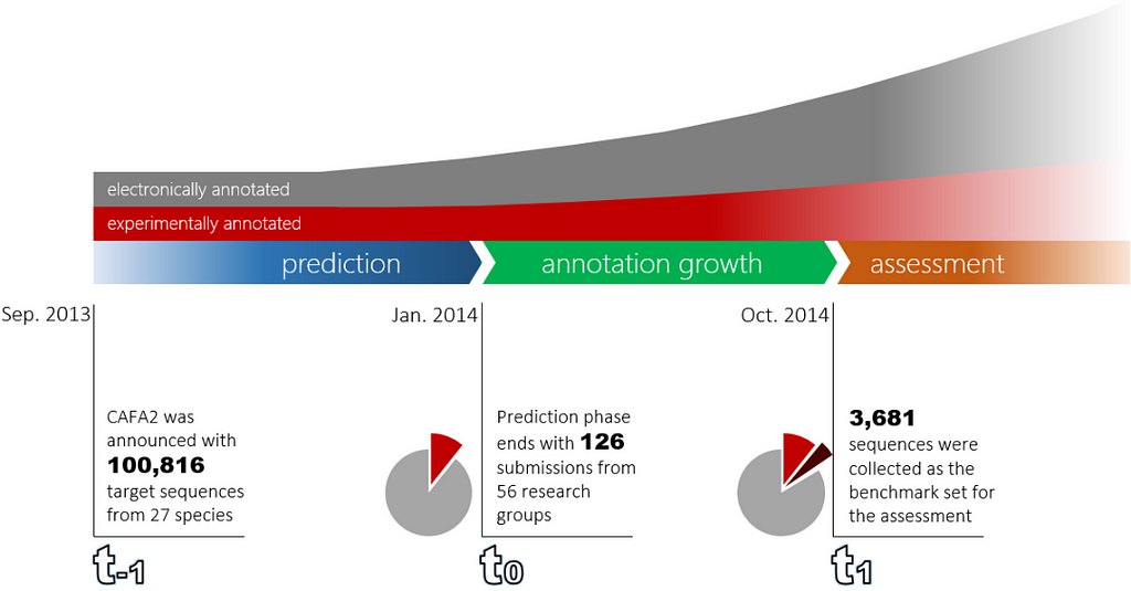
The CAFA competition is a timeline based challenge organized as follows:
- At t_₁ the challenge is announced and the CAFA organizers publish the list of target sequences. For example, CAFA2 was announced in September, 2013.
- t₀ is the deadline for the competing teams to submit the function predictions of the target proteins. The CAFA2 deadline was January, 2014.
- t₀ marks the beginning of an “annotation growth” period where new experimental annotations accumulate on the target proteins. This period lasts around ten months.
- At t₁ (October, 2014 for CAFA2) target sequences with their new experimental annotations are collected and the benchmarks sets are created.
The following figure shows the timeline of the CAFA2 competition:
Annotations
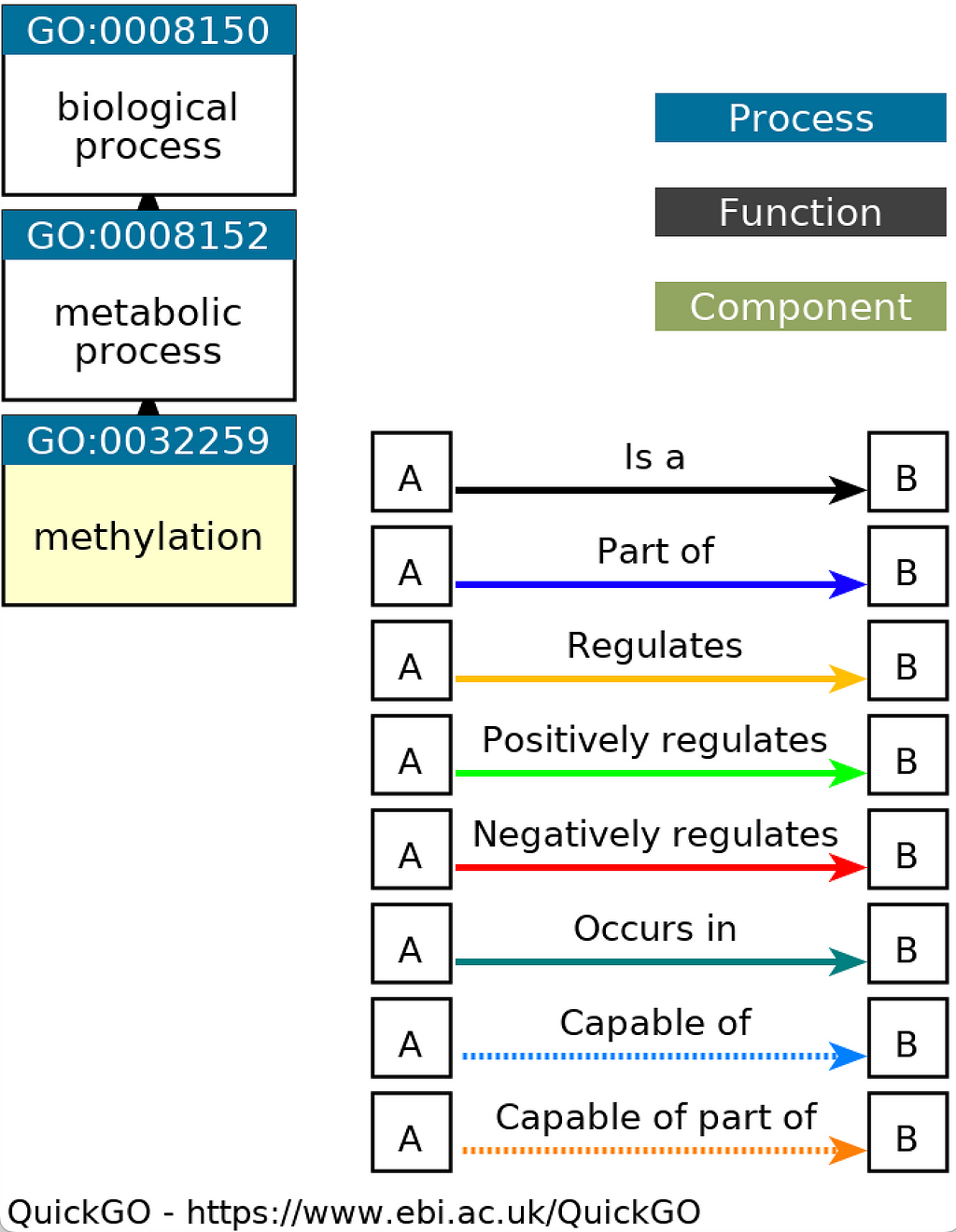
The CAFA competitions use the Gene Ontology (GO) as the mechanism to annotate proteins. The ontology is a set of controlled vocabulary that is used to precisely define a term in question. The GO, in particular, defines terms for three different protein-related aspects (a.k.a. namespaces): the biological process (BP) a protein is related to, the cellular component (CC) and the molecular function (MF) it is related or part of. The GO is an “always evolving” set as new terms are incorporated, refined or made obsolete.
The terms in the GO ontology are organized in a tree structure where each of them is given a unique identifier. The tree structure of the GO allows for linking terms starting from the more generic ones at the top levels of the GO tree to the more specific ones located deeper in the tree. For example, the GO Term “GO:0032259” represents the “Methylation” process which is a type of metabolic process. The following figure obtained from the QuickGO web-based tool shows the representation of “GO:0032259” in the GO tree:
As a result of research experiments, scientists might discover new biological processes, locations or functions that a protein performs. When this happens proteins are annotated with the corresponding GO term and these annotations are then incorporated to the many protein databases such as UniProtKB and UniProt-GOA. For example, the following snippet is the entry for the “Putative methyltransferase 235L” protein (ID: 235L_IIV6) in the UniProtKB/Swiss-Prot database (April, 2021 release) annotated with the “GO:0032259” term mentioned before:
ID   235L_IIV6               Reviewed;         265 AA.
AC   Q91FT7;
DT   16-JUN-2009, integrated into UniProtKB/Swiss-Prot.
...
DR   GO; GO:0008168; F:methyltransferase activity; IEA:UniProtKB-KW.
DR   GO; GO:0032259; P:methylation; IEA:UniProtKB-KW.
...
Benchmark Set
The benchmark is a set of proteins that acquire new experimental annotations during the “annotation growth” period (i.e. between times t₀ and t₁). In other words, the benchmark is generated by recording the annotations present in the source databases at t₁ but missing t₀. The CAFA competition organizers define two types of benchmarks:
- No-Knowledge (NK): This benchmark is composed of proteins that had no experimental annotation in any of the “GO namespaces” and accumulated an experimental annotation between t₀ and t₁.
- Limited-Knowledge (LK): This benchmark is made out of proteins that contain experimental annotations in one or two GO namespaces and acquired new annotations between t₀ and t₁ in a namespace without prior annotations. For example, if a protein with experimental annotations in the MF namespace at t₀ acquires experimental annotations in CC namespace between t₀ and t₁, then it is included the LK benchmark.
Given these classifications there are a total of six benchmarks: two (i.e. NK and LK) for each of the GO ontology namespaces: BP, CC, and MF. In practice, the benchmark files are tab separated value (TSV) files with two columns: the protein ID and the new GO term it has been annotated with. The following is a snippet of the BP-NK benchmark file used for this analysis:
A0A098D6U0  GO:0106150
A0A098D8A0  GO:0106150
A0A163UT06  GO:0051568
A0A1R3RGK0  GO:1900818
A0A1U8QH20  GO:0062032
A0A286LEZ8  GO:0140380
A0A5B9  GO:0002250
A0A5B9  GO:0046631
A0A5B9  GO:0050852
A0JLT2  GO:0032968
...
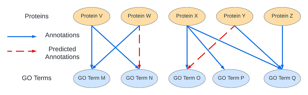
CAFA Competition as a Graph Link Prediction Problem
One way to understand the CAFA competition is as a graph link prediction problem. In this context, we can think of a bipartite graph were there are are two types of nodes: (1) gene products and (2) GO terms. Then, the annotations are the edges of the graph. Based on the graph structure and the properties of the proteins and GO terms, the CAFA competition problem can be reduced to predicting missing links/annotations in the graph:
Methods
This section will go through the steps to generate the training data, benchmark files and the predictors. The tools required are Anaconda, python, git, DVC, the BLAST+ package, and MATLAB.
The initial step to start building the training annotation files and the benchmark is to choose the t₀ and t₁ time points since these determine the release versions of the databases that will be used. At the time this analysis was carried out the latest releases of the databases were the ones of July, 2022. The time points for the benchmark were picked so that the length of the “annotation growth” period was equal to the one used in the CAFA2 challenge (which was approximately 10 months; January to September 2014). Thus, for this analysis:
- t₀: November, 2021
- t₁: July, 2022
Downloading the source code and setting up the Environment
We download the source code and setup our environment to run the necessary scripts:
- Clone the CAFA2 repository and submodules:
git clone --recurse-submodules git@github.com:balvisio/CAFA2.git
cd CAFA2
dvc pull
pushd protein-function-prediction/protein-function-prediction-data/
dvc pull
popd
2. Create and activate a Conda environment:
conda create -n <env-name> python=3.10
conda activate <env-name>
pip install -r requirements.txt
Downloading the Source Databases
In order to build the benchmark set we need to pull information from the following 4 databases:
1. UniProtKB/Swiss-Prot: is a database that contains entries of protein sequences alongside manually annotated functional information such as GO terms. These entries are derived from genome sequencing projects as well as from the research literature².
The latest version of the UniProtKB database and its previous releases can be downloaded from here. For this project I used the following releases:
- version 2021_04: The release from April 2021 since this was the available version released before and closest to t₀. The download link is here and it contains inside the data/text, FASTA and XML formats. The md5 sum of the .tar.gz file is bd2b1b6b0a0027f674017fe5b41fadcb .
- version 2022_02: The release version from February 2022 which is the latest release in July 2022 (t₁) can be downloaded from here. The md5 of the .tar.gz file is c3e8dd5b138f0795aeba2b701982ac2c .
After untaring and unzipping the downloaded databases we obtained the uniprot_sprot.dat files which will be needed to generate the dataset.
2. UniProtKB/TrEMBL: also contains entries of protein sequences but unlike the Swiss-Prot database, the annotations are unreviewed and generated by computational automatic methods². The database in FASTA format can be downloaded from here.
3. Gene Ontology (GO) Database: contains entries for the GO terms that make up the GO. “The GO represents a body of knowledge of the biological domain. Ontologies such as this one usually consist of a set of classes (or terms or concepts) with relations that operate between them.”³ As it was mentioned, the GO is subdivided into three namespaces: molecular function, cellular component, and biological process. The following snippet shows as sample entry from the GO database:
...
[Term]
id: GO:0032259
name: methylation
namespace: biological_process
def: "The process in which a methyl group is covalently attached to a molecule." [GOC:mah]
subset: goslim_chembl
xref: Wikipedia:Methylation
is_a: GO:0008152 ! metabolic process
...
The GO version used to generate the dataset was the one released on October 26th, 2021 and can be downloaded from here. The md5 sum of the file is 6757c819642e79e1406cad3ffcb6ea3d.
4. UniProt-GOA Database: is a database that links the GO database described above with gene products (i.e. genes and any entities encoded by the gene such as protein or functional RNAs). These links are what the Gene Ontology Consortium (GOC) refers to as annotations. The sources of these annotations are collaborating databases and they must contain an evidence code which describes its origin. There are different evidence code categories such as experimental, computational analysis, or electronic³. For a more in-depth explanation and documentation of the GO databases please visit the GOC website.
The GOC publishes two types of UniProt-GOA databases:
- Filtered: “does not contain annotations for those species where a different Consortium group is primarily responsible for providing GO annotations and also excludes annotations made using automated methods.”⁴
- Unfiltered: Contains annotations from a larger number of species and includes automation generated annotations.
The filtered version of the UniProt-GOA database was used since the benchmark sets are concerned with gene products that are experimentally annotated. The UniProt-GOA databases can be obtained from:
- October 26th, 2021 release: The md5 sum of the .gz file is: 6d2be8b48dd0f2505092a8a2cadabd6e .
- July 1st, 2022 release: The md5 sum of the .gz file is: 6f778bdc0b0ea0978e7d75f5e5289064 .
Due to a bug in the build process of these databases (the issue was reported here), the GAF headers are missing. Thus, after downloading the databases the header !gaf-version: 2.0 were added at the beginning of the files.
Filtering and Merging the Source Databases
Once the databases have been downloaded it is necessary to harmonize these different sources of information. The processing steps are:
1. The Uniprot-GOA database contains proteins from both Swiss-Prot and TrEMBL. To improve the efficiency of the scripts that will generate the training datasets and benchmarks, the TrEMBL database is filtered such that only the terms present in the UniProt-GOA are retained. The script protein-function-prediction/preprocessing-scripts/filter_fasta_from_goa.py does this filtering and takes as inputs:
- GAF file: The UniProt-GOA database at time t₀ that will be used to generate the training data.
- FASTA file: for our particular use-case, the TrEMBL database file that needs to be filtered.
The filtering script can be invoked as follows:
python protein-function-prediction/preprocessing-scripts/filter_fasta_from_goa.py \
    <path/to/uniprot-goa-db> \
    <path/to/trembl-db> \
    <path/to/output-filtered-trembl-db>

# Example
python protein-function-prediction/preprocessing-scripts/filter_fasta_from_goa.py \
    uniprot-goa/2021-10-26/goa_uniprot_all_noiea.gaf \
    ~/trembl/uniprot_trembl.fasta \
    uniprotkb/trembl/trembl_seqs_found_in_goa_2021_10_26.fasta
The resulting file is located in uniprotkb/trembl/trembl_seqs_found_in_goa_2021_10_26.fasta .
2. As it is explained in the CAFA2 paper⁵, the benchmark was built from the union of the both the UniProtKB/Swiss-Prot and UniProt-GOA databases. In order to merge the annotations present in these databases we made use of some slightly modified scripts published in the CAFA-Toolset repository.
The steps to merge the annotations from the two databases are:
2.1. Run the Mergedb script to merge the UniProtKB/Swiss-Prot and UniProt-GOA databases at time t₀:
# Run the next two commands only if the file has not been previously uncompressed
tar -xzvf uniprotkb/swiss-prot/2021-04/uniprot_sprot-only2021_04.tar.gz -C uniprotkb/swiss-prot/2021-04/
gunzip uniprotkb/swiss-prot/2021-04/uniprot_sprot.dat.gz

# Mergedb script
python CAFA-Toolset/Mergedb \
  -I1 <path/to/uniprotkb> \
  -I2 <path/to/uniprot-goa> \
  -O <path/to/merged-db>

# Example
python CAFA-Toolset/Mergedb \
  -I1 uniprotkb/swiss-prot/2021-04/uniprot_sprot.dat \
  -I2 uniprot-goa/2021-10-26/goa_uniprot_all_noiea.gaf \
  -O uniprotkb_2021_04_goa_2021_10_26.gaf
2.2. Run the Mergedb script to merge the UniProtKB/Swiss-Prot and UniProt-GOA databases at time t₁. For example:
# Run the next two commands only if the file has not been previously uncompressed
tar -zxvf uniprotkb/swiss-prot/2022-02/uniprot_sprot-only2022_02.tar.gz -C uniprotkb/swiss-prot/2022-02/
gunzip uniprotkb/swiss-prot/2022-02/uniprot_sprot.dat.gz

python CAFA-Toolset/Mergedb \
  -I1 uniprotkb/swiss-prot/2022-02/uniprot_sprot.dat \
  -I2 uniprot-goa/2022-07-01/goa_uniprot_all_noiea.gaf \
  -O uniprotkb_2022_02_goa_2022_07_01.gaf
If you prefer to skip the previous steps, the two GAF files created above are saved in the uniprotkb-goa-merged directory of the CAFA2 repository.
Generating the Training Annotation Files
The training data for the baseline predictors are annotations files that represent an association between a gene products and a GO term. These are TSV files with two columns: the protein sequence ID and the associated GO term:
<sequence ID> <GO term ID>
...
Logically, these annotations have to be built from data that comes from a time point before or equal to t₀. This is done to prevent the “leakage” of data or in other words, giving the predictors information that was not available at the submission time t₀.
At a high level, the creation of the training data involves multiple logical steps:
- Parse the Gene Ontology database and generate a graph where each node represents a GO Term.
- Parse the UniProtKB (Swiss-Prot and TrEMBL) and generate a representation of each the gene products found the databases.
- Extract the annotations from the UniProtKB and merge them with the annotations found in the UniProt-GOA database at t₀.
- Loop through all the annotations found in the previous steps and create a logical link between gene products from step 2 and the GO terms from step 1.
- Propagate all of the associations found in step 4 to all of the GO Term ancestors such that if a gene product was annotated with a particular GO Term there are also an association with each of the parents / more generic GO Terms too.
The code had to handle cases such as:
- GO terms can have alternate IDs and some annotations are mapped to these ones. Thus, additional mappings were necessary to map it to a primary GO term.
- Proteins in UniProtKB can have secondary accessions identifiers so an additional mapping was necessary to always refer to primary one.
- The UniProt-GOA contains entries that belong to the“ComplexPortal” and “RNACentral” databases. These entries were filtered out and not included in the training annotation files.
- The UniProt-GOA contains annotation entries that refer to proteins that are either obsolete or have been move to other databases such as “UniRef” or “UniParc”. The annotations were skipped and not included in the training annotation files.
- Ensure that the annotation files do not contain obsolete GO terms.
All annotations were considered as either:
- electronic when the evidence code was “IEA”.
- manual
The readers are encouraged to read through the source code in protein-function-prediction/deepred/preprocessing/dataset.py to get a deeper understanding of the logic behind the generation of the annotation files.
The steps to create the training annotation files are:
- Creating a “Dataset” file which contains a graph representation of the GO, the gene products and their annotations:
python protein-function-prediction/preprocessing-scripts/create_dataset.py \
    <path/to/GO Ontology/file> \
    <path/to/Swiss-Prot-db-dat-file at t0> \
    <path/to/Swiss-Prot-db-dat-file at t1> \
    <path/to/filtered/TrEMBL-db-fasta file> \
    <path/to/UniProt-GOA-db-gaf-file at t0> \
    <output/dir/to/save/serialized/dataset>

# Example
python protein-function-prediction/preprocessing-scripts/create_dataset.py \
    protein-function-prediction/protein-function-prediction-data/data/ontology/t0/go_20211026.obo \
    protein-function-prediction/protein-function-prediction-data/data/uniprotkb/t0/uniprot_sprot.dat \
    protein-function-prediction/protein-function-prediction-data/data/uniprotkb/t1/uniprot_sprot.dat \
    protein-function-prediction/protein-function-prediction-data/data/trembl/trembl_seqs_found_in_goa_2021_10_26.fasta \
    protein-function-prediction/protein-function-prediction-data/data/goa/t0/goa_uniprot_all_noiea.gaf \
    protein-function-prediction/protein-function-prediction-data/datasets/generic/u-2021-04-g-2021-10-26/
The script will generate a file named dataset.bin in the specified output directory.
2. Create the annotation files using the serialized dataset created in step 1 invoking the create_annotation_files.py script as follows:
python protein-function-prediction/preprocessing-scripts/create_annotation_files.py \
    -f <path/to/dataset/file> \
    <output/dir/to/save/training/annotation/files>

# Example
python protein-function-prediction/preprocessing-scripts/create_annotation_files.py \
    -f protein-function-prediction/protein-function-prediction-data/datasets/generic/u-2021-04-g-2021-10-26/dataset.bin \
    protein-function-prediction/data/annotations/annotations_u_2021_04_g_2021_10_26
The three final annotation files, one for each ontology namespace (i.e. BP, CC, and MF) can be found in the directory protein-function-prediction/data/annotations/annotations_u_2021_04_g_2021_10_26_{bpo|cco|mfo}.tsv . The naming convention of this files are: annotations_u_<UniProtKB_release_date>_g_<UniProt-GOA_release_date>_<ontology>.tsv . In this particular project:
- u_2021_04: UniProt release April, 2021.
- g_2021_10_26: UniProt-GOA release October, 2021.
It might strike as odd to the readers that building the training data requires as input the Swiss-Prot database at t₁ (and right so!). The reason for this requirement is that since the UniProt-GOA was released after UniProt/Swiss-Prot (i.e. October and April, 2021, respectively) certain sequences in UniProt-GOA might not present in the release of the Swiss-Prot database used. Thus, Swiss-Prot at t₁ was used to retrieve those sequences present in UniProt-GOA but missing in Swiss-Prot at t₀.
Building the Benchmark
Using the merged the UniProtKB/Swiss-Prot and UniProt-GOA databases at time points t₀ and t₁ (see the Filtering and Merging the Source Databases section) we invoke the Benchmark script in the CAFA-Toolset repository to build the benchmark. This script takes the two GAF files with the merged annotations as inputs and outputs the benchmark set files in TSV format. This script provides several options to customize the parameters used to build the benchmark set. One of the most important ones is the evidence codes that are considered to be experimental. The CAFA2 paper states that the evidence codes that were considered experimental were: “EXP”, “IDA”, “IPI”, “IMP”, “IGI”, “IEP”, “TAS”, and “IC”.⁵ Thus, to create a benchmark as identical as possible to the one used in the CAFA2 competition, those same evidence codes were passed to the Benchmark script as follows:
python CAFA-Toolset/Benchmark \
    -I1 <path/to/t0/merged/swiss-prot-and-uniprot-goa-file> \
    -I2 <path/to/t1/merged/swiss-prot-and-uniprot-goa-file> \
    --evidence EXP IDA IPI IMP IGI IEP TAS IC \
    -O <output_file_name>

# Example
python CAFA-Toolset/Benchmark \
    -I1 uniprotkb-goa-merged/uniprotkb_2021_04_goa_2021_10_26.gaf \
    -I2 uniprotkb-goa-merged/uniprotkb_2022_02_goa_2022_07_01.gaf \
    --evidence EXP IDA IPI IMP IGI IEP TAS IC \
    -O unfiltered_benchmark_ukb_2021_04_goa_2021_10_26_ukb_2022_02_goa_2022_07_01
The Benchmark script will create a directory named workspace in the directory from which the script is run and inside it will generate the six benchmark files named: <output_file_name>.benchmark_{LK|NK}_{bpo|cco|mfo} .
Given that the training data only contains GO Terms only present at t₀ the script benchmark/filter_annotation_file.py was used to filter out the GO terms created between t₀ and t₁ from the generated benchmark files. In other words, GO Terms that were created in the “annotation growth” period were not included in the benchmark. The benchmark/filter_annotation_file.py script takes as inputs the serialized dataset generated in the Generating the Training Annotation Files section as well as the benchmark file from the last step. Note that this script needs to be run for each of the three benchmark files (i.e. bco , cco , and mfo ) as follows:
python benchmark/filter_annotation_file.py \
    <path/to/serialized/dataset/file> \
    <path/to/unfiltered/benchmark/file> \
    <output/path/to/save/filtered/benchmark/file>

# Example
python benchmark/filter_annotation_file.py \
    protein-function-prediction/protein-function-prediction-data/datasets/generic/u-2021-04-g-2021-10-26/dataset.bin \
    benchmark/u-2021-04-g-2021-10-26-u-2022-02-g-2022-07-01/unfiltered_benchmark_ukb_2021_04_goa_2021_10_26_ukb_2022_02_goa_2022_07_01_NK.bpo \
    benchmark/u-2021-04-g-2021-10-26-u-2022-02-g-2022-07-01/benchmark_ukb_2021_04_goa_2021_10_26_ukb_2022_02_goa_2022_07_01_NK.bpo
The filtered benchmark files can be found in the benchmark/u-2021-04-g-2021-10-26-u-2022-02-g-2022-07-01 directory of the CAFA2 repository.
Build the Query Sequence List
Using the benchmark files we create the following two files:
- Query Sequence List: A text file containing the primary accessions of the sequences found in the benchmark files. This is the list of query sequences against which the predictors will be evaluated.
- Query Sequence FASTA file: The corresponding FASTA file with the query sequences. This file will be used as an input to the BLAST-based predictor to generate predictions and evaluate its performance.
The script query-sequences/generate_query_sequences.sh in the CAFA2 repository generates the two files above. It does the following:
- Reads the protein sequences from a benchmark file.
- Filters out repeated terms.
- If there is any sequence ID which is a secondary accession, it converts it to the primary one.
- Creates the corresponding FASTA file.
It can be invoked as follows:
./query-sequences/generate_query_sequences.sh \
    <path/to/benchmark/file> \
    <path/to/dataset/file> \
    <path/to/save/query/sequence/list/and/fasta/files>

# Example
./query-sequences/generate_query_sequences.sh \
    benchmark/u-2021-04-g-2021-10-26-u-2022-02-g-2022-07-01/benchmark_ukb_2021_04_goa_2021_10_26_ukb_2022_02_goa_2022_07_01_NK.bpo \
    protein-function-prediction/protein-function-prediction-data/datasets/generic/u-2021-04-g-2021-10-26/dataset.bin \
    query-sequences/query_sequences_ukb_2021_04_goa_2021_10_26_ukb_2022_02_goa_2022_07_01_NK.bpo
The generated query sequences files for each of the ontologies can be found in the query-sequences directory.
Building the Baseline Predictors
To compare the performance of predictors it is a standard practice to establish a baseline model which, in many cases, is considered to be logical but maybe simple or naive. For example, if we are trying to create a model that predicts the outside temperature a day into the future, a baseline model could be to predict that the temperature on the next day will be the average temperature of the current day.
The CAFA2 competition established two baseline predictors:
- BLAST-based predictor: It uses the results of a BLAST search to generate predictions. This predictor can be customized to use the resulting percentage of identical parameters (pident) or the BLAST E-value (evalue). For more detailed information please refer to the file matlab/pfp_blast.m in the CAFA2 repository. In this article the “pident” value will be used in the BLAST predictor.
- Naive predictor: It simply predicts a GO term (for all query sequences) with the frequency that it appears in the training data.
The following sections will describe the steps to build both predictors and evaluate them. The predictors will make use of the source databases as well as the training data that were created in previous parts of this article. For the reminder of this article I will use the biological process ontology namespace in the example commands but the steps for the other two ontologies are identical.
Load the Ontology, Ontology Annotation and Query Sequences in MATLAB
After opening the MATLAB console:
- We add the matlab subdirectory of the CAFA2 repository to the MATLAB path:
>> addpath('<path/to/CAFA2/repo>/matlab');2. We build the ontology:
>> ont = pfp_ontbuild(<path/to/ontology/at/t0>);
>>
>> % Example
>> ont = pfp_ontbuild('ontology/t0/go_20211026.obo');
3. We use the ontology from the previous step and the training annotation file to build the training ontology annotation structure:
>> oa = pfp_oabuild(ont{X}, <path/to/training/annotation/file>);
>>
>> % The ontology structure contains 3 cells, one for each ontology:
>> % Biological Process (BP): ont{1}
>> % Cellular Component (CC): ont{2}
>> % Molecular Function (MF): ont{3}
>> %
>> % For example, for the BP ontology annotation:                                                                                                                                                                                                                                                                                                                                                                                                                                                                                                                                                                                  :
>> oa = pfp_oabuild(ont{1}, 'protein-function-prediction/protein-function-prediction-data/data/annotations/annotations_u_2021_04_g_2021_10_26_bpo.tsv');
4. We load the query sequence list text file as a cell array:
>> qseqid = readcell(<path/to/query/sequence/list/file>, 'Filetype', 'text');
>>
>> % Example
>> qseqid = readcell('query-sequences/query_sequences_ukb_2021_04_goa_2021_10_26_ukb_2022_02_goa_2022_07_01_NK.bpo', 'Filetype', 'text');
BLAST-based Predictor
The following subsections will describe the steps needed to build the BLAST-based predictor and generate predictions.
Create the BLAST Database
In order to build the BLAST predictor, we first need to build the BLAST database. This can be achieved by first downloading the BLAST+ package from the NCBI website. The package contains several tools, including makeblastdb which builds a database used by BLAST when performing the search for sequence similarity. The FASTA file we used for creating the BLAST database was a concatenation of the Swiss-Prot database and the filtered TrEMBL database that we created in a previous section:
# Run the following command only if the file has not been previously uncompressed
gunzip uniprotkb/swiss-prot/2021-04/uniprot_sprot.fasta.gz

python uniprotkb/merged-swiss-prot-trembl/merge_dbs_for_blast.py \
    <path/to/swiss-prot-db/fasta/file> \
    <path/to/filtered-trembl-db/fasta/file> \
    <path/to/save/the/merged/databases>

# Example
python uniprotkb/merged-swiss-prot-trembl/merge_dbs_for_blast.py \
    uniprotkb/swiss-prot/2021-04/uniprot_sprot.fasta \
    uniprotkb/trembl/trembl_seqs_found_in_goa_2021_10_26.fasta \
    uniprotkb/merged-swiss-prot-trembl/merged_swiss_prot_2021_04_filtered_trembl_from_goa_2021_10_26.fasta
The concatenated database can be found in uniprotkb/merged-swiss-prot-trembl/merged_swiss_prot_2021_04_filtered_trembl_from_goa_2021_10_26.fasta. Then, to create the BLAST database:
makeblastdb \
    -in <path/to/fasta/file> \
    -title <some_title> \
    -dbtype prot \
    -out <output/path/to/BLAST/database>

# Example
makeblastdb \
    -in uniprotkb/merged-swiss-prot-trembl/merged_swiss_prot_2021_04_filtered_trembl_from_goa_2021_10_26.fasta \
    -title "Merged SwissProt 2021-04 and filtered TrEMBL GOA 2021-10-26" \
    -dbtype prot \
    -out blast/db/merged_swiss_prot_2021_04_filtered_trembl_from_goa_2021_10_26
The BLAST database can be found in the blast/db directory; it is composed by 8 files with the extensions: pdb, pjs , ptf , phr , pot , pto , pin and psq .
Prepare BLAST Results
Having built the BLAST database from the training sequences and the query sequences FASTA files, we have everything we need to evaluate the BLAST predictor. The first step is to blast the query sequences against the training sequences using the following command:
blastp \
    -db <path/to/blast/BLAST/database/file> \
    -query <path/to/query/sequence/list/fasta/file> \
    -outfmt "6 qseqid sseqid evalue length pident nident" \
    -out <path/to/save/blast/search/results>

# Example
blastp \
    -db blast/db/merged_swiss_prot_2021_04_filtered_trembl_from_goa_2021_10_26 \
    -query query-sequences/query_sequences_ukb_2021_04_goa_2021_10_26_ukb_2022_02_goa_2022_07_01_NK.bpo.fasta \
    -outfmt "6 qseqid sseqid evalue length pident nident" \
    -out blast/blastp-results/blastp_ukb_2021_04_goa_2021_10_26_ukb_2022_02_goa_2022_07_01_NK_bpo.blast
The BLAST results are located in the blast/blastp-results directory.
Once we blasted the sequences we load them to MATLAB:
>> B = pfp_importblastp(<path/to/blast/search/results/file>);
>>
>> % Example
>> B = pfp_importblastp('blast/blastp-results/blastp_ukb_2021_04_goa_2021_10_26_ukb_2022_02_goa_2022_07_01_NK_bpo.blast');
and we generate the predictions:
>> blast = pfp_blast(qseqid, B, oa);
Naive Predictor
The only elements required to create a naive predictor are the qseqid cell array and the ontology annotation structure which were created and loaded in previous steps. The predictions of the Naive predictor are generated by:
>> naive = pfp_naive(qseqid, oa);
Creating the submission files from the prediction structures
Once we have the Naive predictor structure we save the results in submission formatted file using the prediction_to_submission_file() function so that it can then be loaded to obtain the evaluation scores:
>> % BLAST
>> prediction_to_submission_file(blast, '<path/to/save/naive/predictions/submission/file>');
>> % Example
>> prediction_to_submission_file(blast, 'blast/blast-predictions/blast_predictions_ukb_2021_04_goa_2021_10_26_ukb_2022_02_goa_2022_07_01_NK_bpo.txt');
>> %
>> %
>> % Naive
>> prediction_to_submission_file(naive, '<path/to/save/naive/predictions/submission/file>');
>> % Example
>> prediction_to_submission_file(naive, 'naive/naive_predictions_ukb_2021_04_goa_2021_10_26_ukb_2022_02_goa_2022_07_01_NK_bpo.txt');
The submission files for the BLAST and Naive predictors can be found in the blast/blast-predictions/and naive/ directories, respectively.
Evaluating the BLAST and Naive Predictors
Once we have generated the CAFA submissions files, we can finally compute the scores of the predictors following the steps described in the README file of the repository. Here we will show how to calculate the fmax score metric of the Naive predictor for the BP ontology. For the BLAST predictor, other ontologies and metrics the commands are almost identical:
- Load the ontology in MATLAB:
>> ont = pfp_ontbuild(<path/to/ontology/at/t0>);
>>
>> % Example
>> ont = pfp_ontbuild('ontology/go_20211026.obo');
- Build the benchmark annotations:
>> oa = pfp_oabuild(ont{1}, '<path/to/benchmark/annotation/file>);
>>
>> % Example
>> oa = pfp_oabuild(ont{1}, 'benchmark/u-2021-04-g-2021-10-26-u-2022-02-g-2022-07-01/benchmark_ukb_2021_04_goa_2021_10_26_ukb_2022_02_goa_2022_07_01_NK.bpo');- Load the predictions:
>> pred = cafa_import(<path/to/prediction/file>, ont{X}, false);
>>
>> % Example
>> pred = cafa_import('naive/naive_predictions_ukb_2021_04_goa_2021_10_26_ukb_2022_02_goa_2022_07_01_NK_bpo.txt', ont{1}, false);- Load the benchmark protein IDs:
>> benchmark = pfp_loaditem(<path/to/query/sequences/list/text/file>, 'char');
>>
>> % Example
>> benchmark = pfp_loaditem('query-sequences/query_sequences_ukb_2021_04_goa_2021_10_26_ukb_2022_02_goa_2022_07_01_NK.bpo', 'char');
- Evaluate the model:
>> fmax = pfp_seqmetric(benchmark, pred, oa, 'fmax');
The steps in this section were coded in the script matlab/evaluate_baseline_predictors.m .
Results
The CAFA2 evaluation code provides various metrics to measure the performance of the predictors such as maximum F-measure (fmax), averaged precision-recall curve (pr), and minimum semantic distance (smin). For more detailed information, please look at the documentation in matlab/pfp_seqmetric.m .
For this article, we evaluated both baseline predictors using the fmax score on the No-Knowledge (NK) benchmark. The following graphs show the performance of the predictors for the three different ontologies. The 95% confidence intervals were computed normal approximated using the bootstrapping method on the benchmark set with 100 iterations (i.e. B=100):
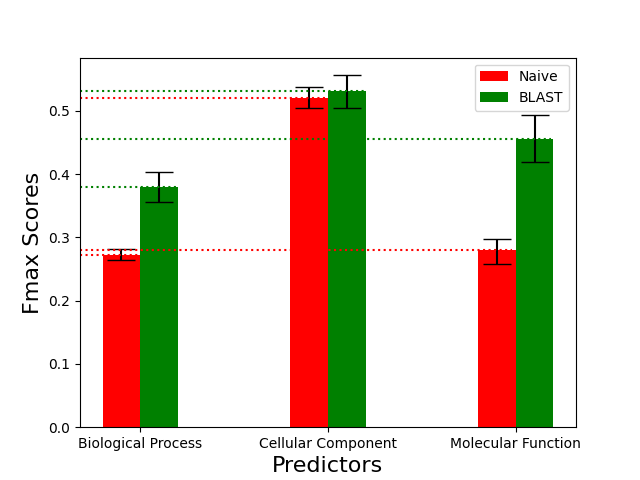
The performance of the baseline predictors greatly varies across the different ontologies. As it is explained in the CAFA2 paper these differences can be the result of (1) topological difference between the GO trees, such as their size and depth, (2) the fact that the BP ontology terms can be considered more abstract than, for example, the CC terms that describe the physical location of a gene product, and (3) the number as well as biases of the annotations in the different ontologies.
The following graphs compare the performance of the Naive and BLAST predictors that were built using the steps described in the Methods section in this article and the ones published in the CAFA2 paper:
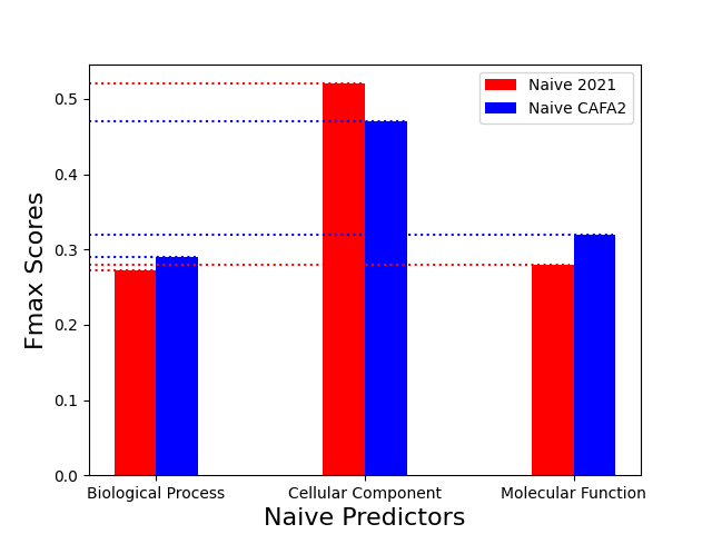
The performance of the Naive predictors across the original CAFA2 benchmark set and one built in this article are very similar. The maximum fmax difference was approximately 0.05. While the Naive 2021 predictor outperformed the CAFA2 predictor in the CC ontology, it underperformed in the BP and MF ones. This shows that additional annotations do not increase the performance of the Naive predictor. The result is expected given the simplistic logic of the predictor based on just the GO terms frequency to predict annotations.
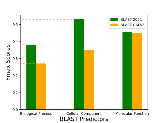
The BLAST predictor built in this article (i.e. BLAST 2021) outperformed the BLAST predictor of the CAFA2 publication by 0.18 and 0.10 in the CC and BP ontologies, respectively. The difference in performance can be attributed to both: (1) additional annotations added between 2014 and 2021 to the source databases, (2) differences in the build process and parameters used in the generation of the BLAST database as well as the benchmark set. Even though further analysis is required to confirm the cause of this observed difference, this benchmark set can be used to compare the performance of more sophisticated predictors.
Conclusion
In this article we have gone through the steps to create a benchmark set and evaluate the performance of protein annotations predictors using the guidelines of the CAFA2 competition. The performance results of the baseline predictors using the newer releases of the source databases are very similar to the ones published in the CAFA2 paper. These results show that the additional annotations incorporated along the years (from 2014 to 2021) to the databases provide no boost in the performance of these simple predictors.
This article provide a very valuable framework to consistently compare the performance of different prediction methods. The steps described can be repeated using future versions of the source databases to assess the change in predictor’s performance as the gene products are annotated with more and newer GO terms.
In following articles I will develop deep learning based predictors and evaluate their performance using the benchmark created in this article. I encourage you to click the “Follow” button to be notified when I publish Part II and III of this series. I have also plans to publish more cool Data Science and ML related articles in the near future. Stay tuned!
Acknowledgements
I would like to thank the creators of the following two repositories on which much of the work in this article is based:
- CAFA2: https://github.com/yuxjiang/CAFA2
- CAFA-Toolset: https://github.com/arkatebi/CAFA-Toolset
References
[1] https://biofunctionprediction.org/cafa/
[2] https://en.wikipedia.org/wiki/UniProt
[3] http://geneontology.org/docs/ontology-documentation/
[4] http://geneontology.org/docs/faq/
[5] Jiang, Y., Oron, T., Clark, W. et al. An expanded evaluation of protein function prediction methods shows an improvement in accuracy. Genome Biol 17, 184 (2016). https://doi.org/10.1186/s13059-016-1037-6
Note on the article images: Unless otherwise noted, all the images were created by the author of this article.
Predicting Protein Functions using Machine Learning was originally published in Towards Data Science on Medium, where people are continuing the conversation by highlighting and responding to this story.
...