

 800+ IT
News
als RSS Feed abonnieren
800+ IT
News
als RSS Feed abonnieren📚 Transformer Aided Supply Chain Network Design
💡 Newskategorie: AI Nachrichten
🔗 Quelle: towardsdatascience.com
Using transformer to help solve a classic problem in supply chain — facility location problem

ChatGPT has been a really hot topic recently due to its general intelligence to accomplish a broad range of tasks. The core model underneath ChatGPT is transformer, which was first proposed for machine translation tasks in the well-known paper Attention is all you need by a research team at Google. Transformer processes an entire sentence at once using an attention mechanism and positional encoding rather than word by word using recursions (like recurrent neural networks). This reduces the information loss during recursions, hence giving transformer a better capability to learn long-range context dependencies, as compared to traditional recurrent neural networks (e.g., LSTM, GRU).
The application of transformer is not limited in language models. Researchers have applied it to many other tasks such as time series forecasting, computer vision, etc., since it was first proposed. A question I have been thinking about is, can transformer be used to help solve practical operations research (OR) problems in supply chain area? In this article, I will show an example of using transformer to assist in solving a classic OR problem in supply chain area — facility location problem.
Facility location problem
Let’s first review the basic setting of this problem. I also briefly discussed about this problem in my first article on Towards Data Science.
Let us assume that a company wants to consider building distribution centers (DCs) among I candidate sites to ship their finished goods to J customers. Each site i has its associate capacity for storing the finished goods with a maximum of m_i units of products. Building a DC on each site i requires a fixed construction fee of f_i. Shipping each unit of product from site i to customer j to incurs a shipping cost of c_ij. Each customer j has a demand of d_j and the demand of all customers must be satisfied. Let binary variable y_i denote whether we build a DC at site i and x_ij denote the volume of products to be shipped from site i to customer j. The optimization problem with an objective to minimize the total cost can be formulated as below:
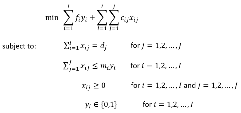
This is a mixed integer linear programming (MILP) problem, which can be solved using any commercial or non-commercial solvers (e.g., CPLEX, GUROBI, SCIP). However, when the model gets large (I and J are large), it could take a long time to solve the model. The main complexity of this problem comes from the integer variables y_i’s, as these variables are the ones that need to be branched on in the branch and bound algorithm. If we can find a faster way to determine the values of y_i’s, that would save a lot of solving time. This is where transformer comes into play.
Transformer aided solution approach
The basic idea of this solution approach is to train a transformer to predict the values of y_i’s by learning from the solutions of a large number of instances of the facility location problem given by a solver. The problem can be formulated as a classification problem as y_i’s can only take values of 0 or 1, corresponding to two classes. Class 0 means site i is not selected for building a DC, and class 1 means site i is selected. The transformer, once trained, can predict which class each y_i belongs to all at once for an unseen instance, thus saving a lot of time spent on branching on integer variables. The diagram below shows the architecture of the transformer adopted here.
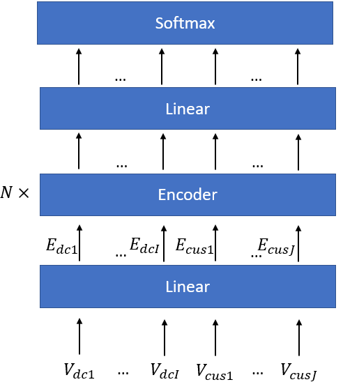
As illustrated by the diagram above, the vector representations of each candidate DC site and customer (containing relevant features of each candidate DC site and customer) are passed into a linear layer. The linear layer produces an embedding vector for each candidate DC site and customer. These embeddings are then passed through N standard encoder blocks as depicted in the paper Attention is all you need. Within the encoder blocks, the multi-head attention mechanism allows each candidate DC site to attend to all the customers’ and other candidate DC sites’ information. Then the outputs of the encoder blocks are passed through a linear layer + softmax layer as the decoding process.
A few accommodations I made to the transformer architecture for this particular problem are:
- Positional encoding is removed due to the fact that the exact order of the input sequence V_dc1, …, V_cusJ does not matter to the output from the perspective of the optimization problem. In other words, randomly shuffling the the input sequence to the transformer shouldn’t affect the solution to the facility location problem.
- The output layer produces a two-dimensional vector for each element in the input sequence V_dc1, …, V_cusJ. The two-dimensional vector contains the probabilities of this element belonging to class 0 and class 1. Note that this two-dimensional vector is actually invalid for elements V_cus1, …, V_cusJ as we cannot build a DC on a customer’s site. So when training the transformer, we mask the outputs corresponding to V_cus1, …, V_cusJ to calculate the loss function, as we don’t care about what these outputs are.
In this facility location problem, we assume that the unit shipping cost c_ij is proportional to the distance between site i and customer j. We define V_dci as [dci_x, dci_y, m_i, f_i, 0], where dci_x and dci_y are the coordinates of candidate DC site i, and 0 indicates that this is a vector representation of the features of a candidate DC site; we define V_cusj as [cusj_x, cusj_y, d_j, 0, 1], where cusj_x and cusj_y are the coordinates of customer j, 0 is the counterpart of f_i in V_dci meaning there’s no fixed fee incurred at a customer, and 1 indicates that this is a vector representation of a customer. Hence each element in the input sequence is a 5-dimensional vector. Through the first linear layer, we project each vector into a high dimensional embedding vector and feed them into the encoder blocks.
To train the transformer, we first need to build a dataset. To set up the labels in the dataset, we solve a large number of instances of the facility location problem using an optimization solver (i.e., SCIP) and then record the values of y_i’s for each instance. The coordinates, d_j’s, m_i’s, f_i’s of each instances are used to construct the input sequence for the transformer. The entire dataset is split into a training set and a test set.
Once the transformer is trained, it can be used to predict which class each candidate DC site i belongs to, in other words, whether y_i is 0 or 1. Then we fix each y_i to its predicted value, and solve the MILP with the rest of the variables x_ij’s. Note that once the values of y_i’s are fixed, the facility location problem becomes an LP, which is much easier to solve using the optimization solver. The resulting solution may be sub-optimal, but saves a lot of solving time for large instances.
One caveat of the transformer aided solution approach is that the predicted y_i values given by the transformer may sometimes result in infeasibility for the MILP, due to the fact that the predictions of the transformer are not perfectly accurate. The infeasibility is caused by the sum of m_i * y_i being smaller than the sum of d_j, meaning there will not be enough supply to satisfy the total demand across all the customers if we follow the predicted values of y_i’s. In such cases, we retain the y_i values where y_i is 1, and search through the rest of the candidate DC sites to make up the difference between the total supply and demand. Essentially, we need to solve another optimization problem as below:
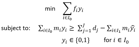
Here, I_0 is the set of candidate DC sites of which the predicted y_i value is 0 and I_1 is the set of candidate DC sites of which the predicted y_i value is 1. This is essentially a knapsack problem which can be solved by an optimization solver. However, with large instances, this problem could still consume a lot of solving time. Hence, I decided to adopt a heuristic to solve this problem — the greedy algorithm for solving fractional knapsack problems. Specifically, we calculate the ratio f_i/m_i for each candidate DC site in I_0, and sort the sites in an ascending order based on the ratios. Then we select the sites from the first to the last one by one until the constraint is met. After this procedure, the y_i values of the selected sites in I_0, together with all the sites in I_1, are set to 1. The y_i values of the rest sites are set to 0. This configuration is then fed into the optimization solver to solve for the rest x_ij variables.
Numerical experiments
I randomly created 800 instances of the facility location problem with 100 candidate DC sites and 200 customers. I used 560 instances of them for training and 240 instances for testing. The non-commercial solver SCIP was adopted for solving the instances. The code for generating the instances is given below.
from pyscipopt import Model, quicksum
import numpy as np
import pickle

rnd = np.random
models_output = []
for k in range(1000):
    info = {}
    np.random.seed(k)
    n_dc = 100
    n_cus = 200
    c = []
    loc_x_dc = rnd.rand(n_dc)*100
    loc_y_dc = rnd.rand(n_dc)*100
    loc_x_cus = rnd.rand(n_cus)*100
    loc_y_cus = rnd.rand(n_cus)*100
    xy_dc = [[x,y] for x,y in zip(loc_x_dc,loc_y_dc)]
    xy_cus = [[x,y] for x,y in zip(loc_x_cus,loc_y_cus)]
    for i in xy_dc:
        c_i = []
        for j in xy_cus:
            c_i.append(np.sqrt((i[0]-j[0])**2 + (i[1]-j[1])**2)*0.01)
        c.append(c_i)

    f= []
    m = []
    d = []

    for i in range(n_dc):
        f_rand = np.round(np.random.normal(100,15))
        if f_rand < 40:
            f.append(40)
        else:
            f.append(f_rand)
        m_rand = np.round(np.random.normal(70,10))
        if m_rand < 30:
            m.append(30)
        else:
            m.append(m_rand)
    for i in range(n_cus):
        d_rand = np.round(np.random.normal(20,5))
        if d_rand < 5:
            d.append(5)
        else:
            d.append(d_rand)

    f = np.array(f)
    m = np.array(m)
    d = np.array(d)
    c = np.array(c)

    model = Model("facility selection")
    x,y = {},{}
    x_names = ['x_'+str(i)+'_'+str(j) for i in range(n_dc) for j in range(n_cus)]
    y_names = ['y_'+str(i) for i in range(n_dc)]
    for i in range(n_dc):
        for j in range(n_cus):
            x[i,j] = model.addVar(name=x_names[i*n_cus+j])
    for i in range(n_dc):
        y[i] = model.addVar(name=y_names[i],vtype='BINARY')
    model.setObjective(quicksum(f[i]*y[i] for i in range(n_dc))+quicksum(c[i,j]*x[i,j] for i in range(n_dc) for j in range(n_cus)), 'minimize')
    for j in range(n_cus):
        model.addCons(quicksum(x[i,j] for i in range(n_dc)) == d[j])
    for i in range(n_dc):
        model.addCons(quicksum(x[i,j] for j in range(n_cus)) <= m[i]*y[i])
    model.optimize()

    y_sol = []
    for i in range(n_dc):
        y_sol.append(model.getVal(y[i]))
    x_sol = []
    for i in range(n_dc):
        x_i = []
        for j in range(n_cus):
            x_i.append(model.getVal(x[i,j]))
        x_sol.append(x_i)
    obj_vol = model.getObjVal()

    info['f'] = f
    info['m'] = m
    info['d'] = d
    info['c'] = c
    info['y'] = y_sol
    info['x'] = x_sol
    info['obj'] = obj_vol
    info['xy_dc'] = xy_dc
    info['xy_cus'] = xy_cus
    models_output.append(info)

with open('models_output.pkl', 'wb') as outp:
    pickle.dump(models_output, outp)
Then we read in the solutions and create the dataset used for training the transformer. Note that here I converted the cartesian coordinate system into polar coordinate system when building the dataset, as the latter one leads to higher accuracy for the transformer.
from sklearn.preprocessing import MinMaxScaler
import torch

with open('models_output.pkl', 'rb') as f:
    models_output = pickle.load(f)

def convert_coord(xy):
    r = np.sqrt((xy[0]-50)**2 + (xy[1]-50)**2)
    theta = np.arctan2(xy[1],xy[0])
    return [theta, r]

dataset = []
for k in range(len(models_output)):
    data = {}
    xy_site = []
    new_xy_dc = [convert_coord(i) for i in models_output[k]['xy_dc']]
    new_xy_cus = [convert_coord(i) for i in models_output[k]['xy_cus']]
    xy_site.extend(new_xy_dc)
    xy_site.extend(new_xy_cus)
    d_site = []
    d_site.extend([[i] for i in models_output[k]['m']])
    d_site.extend([[i] for i in models_output[k]['d']])
    f_site = []
    f_site.extend([[i] for i in models_output[k]['f']])
    f_site.extend([[0] for i in range(200)])
    i_site = []
    i_site.extend([[0] for i in range(100)])
    i_site.extend([[1] for i in range(200)])
    x = np.concatenate((xy_site, d_site), axis=1)
    x = np.concatenate((x, f_site), axis=1)
    x = np.concatenate((x, i_site), axis=1)
    if k == 0:
        scaler_x = MinMaxScaler()
        x = scaler_x.fit_transform(x)
    else:
        x = scaler_x.transform(x)
    x = np.expand_dims(x,axis=1)
    y = []
    y_cus = [2 for i in range(200)]
    y.extend(models_output[k]['y'])
    y.extend(y_cus)
    x = torch.from_numpy(x).float()
    y = torch.from_numpy(np.array(y)).long()
    data['x'] = x
    data['y'] = y
    dataset.append(data)
    mask = []
    mask_true = [True for i in range(100)]
    mask_false = [False for i in range(200)]
    mask.extend(mask_true)
    mask.extend(mask_false)
Then we define the architecture of the transformer. Here the embedding vectors are 256-dimensional, the number of heads in the multi-head attention mechanism is 8, and the number of encoder blocks is 3. I didn’t experiment with many hyper-parameter settings as this setting already achieved satisfactory accuracy. More hyper-parameter tuning can be done to further increase the accuracy of the transformer.
import torch
from torch import nn, Tensor
import torch.nn.functional as F
from torch.nn import TransformerEncoder, TransformerEncoderLayer

class TransformerModel(nn.Module):
    def __init__(self, n_class=2, d_input=5, d_model=256, nhead=8, d_hid=256, nlayers=3, dropout=0.5):
        super().__init__()
        encoder_layers = TransformerEncoderLayer(d_model, nhead, d_hid, dropout)
        self.transformer_encoder = TransformerEncoder(encoder_layers, nlayers)
        self.d_model = d_model
        self.encoder = nn.Linear(d_input, d_model)
        self.decoder = nn.Linear(d_model, n_class)

        self.init_weights()

    def init_weights(self) -> None:
        initrange = 0.1
        self.decoder.weight.data.uniform_(-initrange, initrange)


    def forward(self, src: Tensor) -> Tensor:
        src = self.encoder(src)
        output = self.transformer_encoder(src)
        output = self.decoder(output)
        return output
Then we train and test the transformer with the dataset created previously.
import torch.optim as optim

def acc(y_pred, y_test):
    y_pred_softmax = torch.log_softmax(y_pred, dim = 1)
    _, y_pred_tags = torch.max(y_pred_softmax, dim = 1)
    correct_pred = (y_pred_tags == y_test).float()
    acc = correct_pred.sum() / len(correct_pred)
    return acc

LEARNING_RATE = 0.0001
EPOCHS = 100
model = TransformerModel()
criterion = nn.CrossEntropyLoss()
optimizer = optim.Adam(model.parameters(), lr=LEARNING_RATE)
n_class = 2

for e in range(1,EPOCHS+1):
    model.train()
    e_train_loss = []
    e_train_acc = []
    for i in range(560):
        optimizer.zero_grad()
        y_pred = model(dataset[i]['x'])
        train_loss = criterion(y_pred.view(-1,n_class)[mask], dataset[i]['y'][mask])
        train_acc = acc(y_pred.view(-1,n_class)[mask], dataset[i]['y'][mask])
        train_loss.backward()
        optimizer.step()
        e_train_loss.append(train_loss.item())
        e_train_acc.append(train_acc.item())
    with torch.no_grad():
        model.eval()
        e_val_loss = []
        e_val_acc = []
        for i in range(560,800):
            y_pred = model(dataset[i]['x'])
            val_loss = criterion(y_pred.view(-1,n_class)[mask], dataset[i]['y'][mask])
            val_acc = acc(y_pred.view(-1,n_class)[mask], dataset[i]['y'][mask])
            e_val_loss.append(val_loss.item())
            e_val_acc.append(val_acc.item())
    print('epoch:', e)
    print('train loss:', np.mean(e_train_loss))
    print('train acc:', np.mean(e_train_acc))
    print('val loss:', np.mean(e_val_loss))
    print('val acc:', np.mean(e_val_acc))

torch.save(model.state_dict(), desired_path)
After training, the transformer achieved approximately 92% accuracy on the test set containing 240 instances. Considering the test set is not imbalanced (46.57% and 53.43% of the labels in the test set are 0 and 1 respectively) and our transformer is not always predicting the same class, 92% accuracy should be a satisfactory score.
Finally, we test the transformer aided solution approach for the facility location problem vs solving the MILP directly using the SCIP solver only. The main purpose is to prove that the transformer helps reduce a lot of solving time without a significant deterioration in the solution quality.
I created another 100 random unseen instances with m_i, f_i, d_j parameters following the same distribution as those instances used for training the transformer, and applied each solution approach to them. I tested for 3 cases with different numbers of candidate DC sites and customers, namely (n_dc=100,n_cus=200), (n_dc=200,n_cus=400), (n_dc=400,n_cus=800). The code is given below.
import time
from bisect import bisect

def resolve_infeasibility(m,f,d,y):
    idx = np.arange(len(y))
    idx = idx[y==0]
    m = m[idx]
    f = f[idx]
    r = f/m
    r_idx = np.argsort(r)
    m_sort = m[r_idx]
    idx = idx[r_idx]
    m_sort_sum = np.cumsum(m_sort)
    up_to_idx = bisect(m_sort_sum,d)
    idx = idx[:up_to_idx+1]
    for i in idx:
        y[i] = 1
    return y

transformer_model = TransformerModel()
transformer_model.load_state_dict(torch.load(desired_path))

obj_transformer = []
gap_transformer = []
time_transformer = []
obj_original = []
gap_original = []
time_original = []

rnd = np.random

for k in range(800,900):
    np.random.seed(k)
    n_dc = 100
    n_cus = 200
    c = []
    loc_x_dc = rnd.rand(n_dc)*100
    loc_y_dc = rnd.rand(n_dc)*100
    loc_x_cus = rnd.rand(n_cus)*100
    loc_y_cus = rnd.rand(n_cus)*100
    xy_dc = [[x,y] for x,y in zip(loc_x_dc,loc_y_dc)]
    xy_cus = [[x,y] for x,y in zip(loc_x_cus,loc_y_cus)]
    for i in xy_dc:
        c_i = []
        for j in xy_cus:
            c_i.append(np.sqrt((i[0]-j[0])**2 + (i[1]-j[1])**2)*0.01)
        c.append(c_i)

    f= []
    m = []
    d = []

    for i in range(n_dc):
        f_rand = np.round(np.random.normal(100,15))
        if f_rand < 40:
            f.append(40)
        else:
            f.append(f_rand)
        m_rand = np.round(np.random.normal(70,10))
        if m_rand < 30:
            m.append(30)
        else:
            m.append(m_rand)
    for i in range(n_cus):
        d_rand = np.round(np.random.normal(20,5))
        if d_rand < 5:
            d.append(5)
        else:
            d.append(d_rand)

    f = np.array(f)
    m = np.array(m)
    d = np.array(d)
    c = np.array(c)

    start_time = time.time()
    model = Model("facility selection")
    x,y = {},{}
    x_names = ['x_'+str(i)+'_'+str(j) for i in range(n_dc) for j in range(n_cus)]
    y_names = ['y_'+str(i) for i in range(n_dc)]
    for i in range(n_dc):
        for j in range(n_cus):
            x[i,j] = model.addVar(name=x_names[i*n_cus+j])
    for i in range(n_dc):
        y[i] = model.addVar(name=y_names[i],vtype='BINARY')
    model.setObjective(quicksum(f[i]*y[i] for i in range(n_dc))+quicksum(c[i,j]*x[i,j] for i in range(n_dc) for j in range(n_cus)), 'minimize')
    for j in range(n_cus):
        model.addCons(quicksum(x[i,j] for i in range(n_dc)) == d[j])
    for i in range(n_dc):
        model.addCons(quicksum(x[i,j] for j in range(n_cus)) <= m[i]*y[i])
    model.optimize()
    time_original.append(time.time()-start_time)
    obj_original.append(model.getObjVal())
    gap_original.append(model.getGap())

    start_time = time.time()
    xy_site = []
    new_xy_dc = [convert_coord(i) for i in xy_dc]
    new_xy_cus = [convert_coord(i) for i in xy_cus]
    xy_site.extend(new_xy_dc)
    xy_site.extend(new_xy_cus)
    d_site = []
    d_site.extend([[i] for i in m])
    d_site.extend([[i] for i in d])
    f_site = []
    f_site.extend([[i] for i in f])
    f_site.extend([[0] for i in range(200)])
    i_site = []
    i_site.extend([[0] for i in range(100)])
    i_site.extend([[1] for i in range(200)])
    x = np.concatenate((xy_site, d_site), axis=1)
    x = np.concatenate((x, f_site), axis=1)
    x = np.concatenate((x, i_site), axis=1)
    x = scaler_x.transform(x)
    x = np.expand_dims(x,axis=1)
    x = torch.from_numpy(x).float()

    transformer_model.eval()
    y_pred = transformer_model(x)
    y_pred_softmax = torch.log_softmax(y_pred.view(-1,2)[mask], dim = 1)
    _, y_pred_tags = torch.max(y_pred_softmax, dim = 1)
    if np.sum(m*y_pred_tags.numpy()) < np.sum(d):
        y_pred_corrected = resolve_infeasibility(m,f,np.sum(d)-np.sum(m*y_pred_tags.numpy()),y_pred_tags.numpy())
    else:
        y_pred_corrected = y_pred_tags.numpy()

    model = Model("facility selection with transformer")
    x,y = {},{}
    x_names = ['x_'+str(i)+'_'+str(j) for i in range(n_dc) for j in range(n_cus)]
    y_names = ['y_'+str(i) for i in range(n_dc)]
    for i in range(n_dc):
        for j in range(n_cus):
            x[i,j] = model.addVar(name=x_names[i*n_cus+j])

    for i in range(n_dc):
        if y_pred_corrected[i] == 1:
            y[i] = model.addVar(name=y_names[i],vtype='BINARY',lb=1)
        else:
            y[i] = model.addVar(name=y_names[i],vtype='BINARY',ub=0)
    model.setObjective(quicksum(f[i]*y[i] for i in range(n_dc))+quicksum(c[i,j]*x[i,j] for i in range(n_dc) for j in range(n_cus)), 'minimize')
    for j in range(n_cus):
        model.addCons(quicksum(x[i,j] for i in range(n_dc)) == d[j])
    for i in range(n_dc):
        model.addCons(quicksum(x[i,j] for j in range(n_cus)) <= m[i]*y[i])
    model.optimize()
    time_transformer.append(time.time()-start_time)
    obj_transformer.append(model.getObjVal())
    gap_transformer.append(model.getGap())
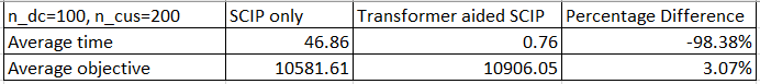
The average solving time (unit: seconds, on a laptop with Intel(R) Core(TM) i7–10750H CPU, 6 cores) and objective value of each solution approach for each case are reported in the table below.
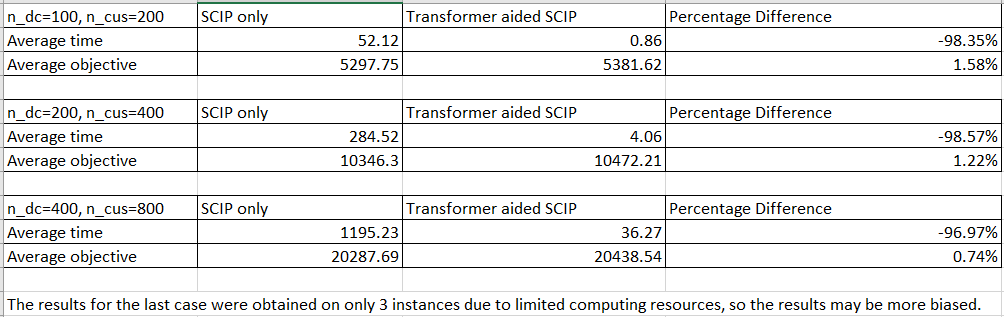
We can see that for all cases, the transformer aided solution approach consumes around 2% of the solving time of the SCIP only solution approach, while the objective value deteriorates by only around 1%.
So far we have only tested the transformer aided solution approach on instances with parameters following the same distribution as the training set. What if we apply it to instances with parameters following a different distribution? To test this, I generated 100 test instances for (n_dc=100,n_cus=200) with m_i, f_i, d_j parameters following a normal distribution with double mean and double standard deviation, using the code below.
f = []
m = []
d = []

for i in range(n_dc):
    f_rand = np.round(np.random.normal(200,30))
    if f_rand < 80:
        f.append(80)
    else:
        f.append(f_rand)
    m_rand = np.round(np.random.normal(140,20))
    if m_rand < 60:
        m.append(60)
    else:
        m.append(m_rand)
for i in range(n_cus):
    d_rand = np.round(np.random.normal(40,10))
    if d_rand < 10:
        d.append(10)
    else:
        d.append(d_rand)
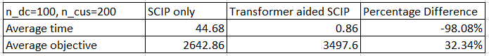
The results obtained from these instances are reported in the table below.
We see that the transformer aided solution approach consumes around 2% of the solving time of the SCIP only solution approach, while the objective value deteriorates by around 3%, a little bit more than the previous test, but still acceptable.
We generate one more set of 100 test instances with m_i, f_i, d_j parameters following a normal distribution with half mean and standard deviation, using the code below.
f = []
m = []
d = []

for i in range(n_dc):
    f_rand = np.round(np.random.normal(50,7.5))
    if f_rand < 20:
        f.append(20)
    else:
        f.append(f_rand)
    m_rand = np.round(np.random.normal(35,5))
    if m_rand < 15:
        m.append(15)
    else:
        m.append(m_rand)
for i in range(n_cus):
    d_rand = np.round(np.random.normal(10,2.5))
    if d_rand < 3:
        d.append(3)
    else:
        d.append(d_rand)
The results are reported in the table below.
We see that the transformer aided solution approach still greatly saves the solving time, however, there is also a significant deterioration in solution quality. So the transformer is indeed a bit overfitted to the parameter distributions of the instances in the training set.
Conclusions
In this article, I trained a transformer model to help solve a classic MILP in supply chain area — facility location problem. The transformer is able to predict the correct values the integer variables should take by learning through the solutions of hundreds of instances given by SCIP. We then fix the integer variables in the SCIP solver to the predicted values given by the transformer model and solve for the rest variables. Numerical experiments show that the transformer aided solution approach reduces the solving time significantly with only slight deterioration in solution quality, when applied to instances with parameters following the same or similar distributions.
Applying machine learning (ML) to help solve MILPs faster is an emerging research topic in both ML and OR communities, as mentioned in my first article. Existing research ideas include supervised learning (learning from a solver) and reinforcement learning (learning to solve MILPs itself by exploring the solution space and observing rewards), etc. The core idea of this article belongs to the former class (supervised learning), and takes advantage of the attention mechanism in the transformer model to learn making decisions for the integer variables. Since the transformer model learns from the solver, the solution quality of the transformer aided solution approach can never surpass the solver, but we gain a huge saving in the solving time.
Using a pre-trained ML model to generate partial solutions for MILPs could be a promising idea to expedite the solving process for large instances in commercial applications. Here, I selected the facility location problem as an example of MILPs to do experiments, but the same idea applies to other problems, such as assignment problems. This approach is best suited for the case where we want to repeatedly solve large MILP instances with parameters following the same or similar distributions, as the pre-trained ML model tends to be overfitted to the parameter distributions in the training instances. One way to improve the robustness of this approach may be to include more instances with parameters following more diverse distributions to reduce overfitting, and this can be something to explore in my future articles.
Thanks for reading!
Transformer Aided Supply Chain Network Design was originally published in Towards Data Science on Medium, where people are continuing the conversation by highlighting and responding to this story.
...