

 800+ IT
News
als RSS Feed abonnieren
800+ IT
News
als RSS Feed abonnieren📚 The Job-Shop Scheduling Problem: Mixed-Integer Programming Models
💡 Newskategorie: AI Nachrichten
🔗 Quelle: towardsdatascience.com
Mathematical modeling and Python implementation of the classical sequencing problem using Pyomo

The job-shop scheduling problem (JSSP) is a widely studied optimization problem with several industrial applications. The goal is to define how to minimize the makespan required to allocate shared resources (machines) over time to complete competing activities (jobs). As for other optimization problems, mixed-integer programming can be an effective tool to provide good solutions, although for large-scale instances one should probably resort to heuristics.
Throughout this article, one may find two of the most usual mixed-integer programming formulations for the JSSP with implementation in Python, using the pyomo library (Bynum et al., 2021). Those interested in details can follow along with the complete code available in this git repository.
If you are unfamiliar with mixed-integer programming or optimization in general, you might have a better experience after reading this introduction on the subject.
An introduction to mixed-integer linear programming: The knapsack problem
Now let us dive in!
Problem statement
Suppose a set of jobs J needs to be processed in a set of machines M, each in a given order. For instance, job number 1 might need to be processed in machines (1, 4, 3, 2), whereas job number 2 in (2, 3, 4, 1). In this case, before going to machine 4, job 1 must have gone to machine 1. Analogously, before going to machine 1, job 2 must have been processed in machine 4.
Each machine can process only one job at a time. Operations are defined by pairs (machine, job) and each has a specific processing time p. Therefore, the total makespan depends on how one allocates resources to perform tasks.
The figure below illustrates an optimal sequence of operations for a simple instance with 5 machines and 4 jobs. Notice that each machine processes just one job at a time and each job is processed by only one machine at a time.
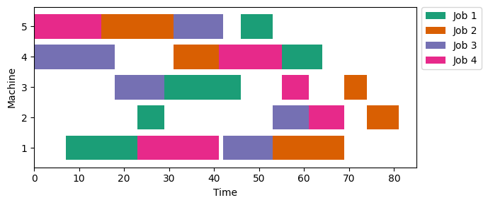
As for other optimization problems, we must convert these rules into mathematical equations to obtain smart allocations of resources. Therefore, in the following section, let us see two usual formulations for the JSSP.
Mixed-integer models
Following the study of Ku & Beck (2016), two formulations for the JSSP will be presented: the disjunctive model (Manne, 1960) and the time-index model (Bowman, 1959; Kondili, 1993). Those interested might refer to Wagner (1959) for a third formulation (rank-based). The disjunctive model is surely the most efficient of the three for the original problem. However, others might be easier to handle when incorporating new constraints that might occur in real-world problems.
In the disjunctive model, let us consider a set J of jobs and a set M of machines. Each job j must follow a processing order (σʲ₁, σʲ₂, …, σʲₖ) and each operation (m, j) has a processing time p. The decision variables considered are the time that job j starts on machine m, xₘⱼ; a binary that marks precedence of job i before j on machine m, zₘᵢⱼ; and the total makespan of operation, C, which is itself the minimization objective.
We need to create constraints to ensure that:
- The starting time of job j in machine m must be greater than the starting time of the previous operation of job j plus its processing time.
- Each machine processes just one job at a time. To do this, we state that if i precedes j in machine m, the starting time of job j in machine m must be greater than or equal to the starting time of job i plus its processing time.
- Of every pair of jobs i, j one element must precede the other for each machine m in M.
- The total makespan is greater than the starting time of every operation plus its processing time.
And we get the following formulation:

In which, V is an arbitrarily large value (big M) of the “either-or” constraint.
The next formulation explored will be the time-indexed model. It is limited in the sense that only integer processing times can be considered and one can notice that it produces a constraint matrix with several nonzero elements, which makes it computationally more expensive than the disjunctive model. Furthermore, as processing times increase, the number of decision variables increases as well.
In the time-indexed model, we will consider the same sets of jobs J and machines M, besides a set of discrete intervals T. The choice of the size of T might be oriented in the same way as the definition of V: the sum of all processing times. The same parameters of the order of jobs and processing times will be used too. However, in this approach, we only consider binary variables that mark it job j starts at machine m at instant t, xₘⱼₜ, besides the real-valued (or integer) makespan C.
Let us formulate the constraints:
- Each job j at machine m starts only once.
- Ensure that each machine processes just one job at a time. And this is the hard one in the time-indexed approach. To do this, we state that at most one job j can start at machine m during the time span between the current time t and pₘⱼ previous times. For each machine and time instant.
- The starting time of job j in machine m must be greater than the starting time of the previous operation of job j plus its processing time.
- The total makespan is greater than the starting time of every operation plus its processing time.

Implementation
Before diving into the models, let us create a few utility classes to handle the parameters of this problem. The first will be JobSequence a Python list child class with methods to find previous and following elements in a sequence. This will be useful when referring to the sequence of machines for each job.
class JobSequence(list):

    def prev(self, x):
        if self.is_first(x):
            return None
        else:
            i = self.index(x)
            return self[i - 1]

    def next(self, x):
        if self.is_last(x):
            return None
        else:
            i = self.index(x)
            return self[i + 1]

    def is_first(self, x):
        return x == self[0]

    def is_last(self, x):
        return x == self[-1]

    def swap(self, x, y):
        i = self.index(x)
        j = self.index(y)
        self[i] = y
        self[j] = x

    def append(self, __object) -> None:
        if __object not in self:
            super().append(__object)
        else:
            pass
Now let us create a white-label class for parameters. It must store the set of jobs J, the set of machines M, the sequence of operations of each job j in a dict of JobSequences, and the processing time of each pair m, j in a tuple-index dictionary p_times.
class JobShopParams:

    def __init__(self, machines, jobs, p_times, seq):
        self.machines = machines
        self.jobs = jobs
        self.p_times = p_times
        self.seq = seq
And at last, a class to generate random problem instances from a given number of machines, jobs, and interval of processing times.
import numpy as np


class JobShopRandomParams(JobShopParams):

    def __init__(self, n_machines, n_jobst, t_span=(1, 20), seed=None):

        self.t_span = t_span
        self.seed = seed

        machines = np.arange(n_machines, dtype=int)
        jobs = np.arange(n_jobs, dtype=int)
        p_times = self._random_times(machines, jobs, t_span)
        seq = self._random_sequences(machines, jobs)
        super().__init__(machines, jobs, p_times, seq)

    def _random_times(self, machines, jobs, t_span):
        np.random.seed(self.seed)
        t = np.arange(t_span[0], t_span[1])
        return {
            (m, j): np.random.choice(t)
            for m in machines
            for j in jobs
        }

    def _random_sequences(self, machines, jobs):
        np.random.seed(self.seed)
        return {
            j: JobSequence(np.random.permutation(machines))
            for j in jobs
        }
Now we can instantiate random problems at ease to validate our models.
In the following steps, we will create three classes that inherit from pyomo’s ConcreteModel. The first will be a white-label class for the MIP models. The second and the third will be the disjunctive and time-indexed model classes respectively.
import pyomo.environ as pyo


class JobShopModel(pyo.ConcreteModel):

    def __init__(self, params, **kwargs):
        super().__init__()
        self.params = params
        self._construct_sets()
        self._construct_params()

    @property
    def seq(self):
        return self.params.seq

    def _construct_sets(self):
        self.M = pyo.Set(initialize=self.params.machines)
        self.J = pyo.Set(initialize=self.params.jobs)

    def _construct_params(self):
        self.p = pyo.Param(self.M, self.J, initialize=self.params.p_times)
        self.V = sum(self.p[key] for key in self.p)
One can notice the sets of jobs J and machines M are stored in the instance attributes of the same name. The attribute p holds processing times, and V is the reasonable upper limit for makespan.
Let us now create the disjunctive model, the DisjModel class.
class DisjModel(JobShopModel):

    def __init__(self, params, **kwargs):
        super().__init__(params, **kwargs)
        self._create_vars()
        self._create_cstr()
        self.obj = pyo.Objective(rule=self.C, sense=pyo.minimize)

    def _create_vars(self):
        self.x = pyo.Var(self.M, self.J, within=pyo.NonNegativeReals)
        self.z = pyo.Var(self.M, self.J, self.J, within=pyo.Binary)
        self.C = pyo.Var(within=pyo.NonNegativeReals)

    def _create_cstr(self):
        self.cstr_seq = pyo.Constraint(self.M, self.J, rule=cstr_seq)
        self.cstr_precede = pyo.Constraint(self.M, self.J, self.J, rule=cstr_precede)
        self.cstr_comp_precede = pyo.Constraint(self.M, self.J, self.J, rule=cstr_comp_precede)
        self.cstr_total_time = pyo.Constraint(self.J, rule=cstr_total_time)
Instances of DisjModel carry attributes x, z, and C — of the variables previously described. The objective is quite simple: minimize one of the decision variables: C. And notice we still need to define rules for the constraints. They are defined in the same order previously listed when introducing the model. Let us now write them in pyomo style.
def cstr_seq(model, m, j):
    o = model.seq[j].prev(m)
    if o is not None:
        return model.x[o, j] + model.p[o, j] <= model.x[m, j]
    else:
        return pyo.Constraint.Skip


def cstr_precede(model, m, j, k):
    if j != k:
        return model.x[m, j] + model.p[m, j] <= model.x[m, k] + model.V * (1 - model.z[m, j, k])
    else:
        return pyo.Constraint.Skip


def cstr_comp_precede(model, m, j, k):
    if j != k:
        return model.z[m, j, k] + model.z[m, k, j] == 1
    else:
        return model.z[m, j, k] == 0


def cstr_total_time(model, j):
    m = model.seq[j][-1]
    return model.x[m, j] + model.p[m, j] <= model.C
And we are ready to solve JSSP problems with the disjunctive model approach. Let us define the time-indexed model as well.
class TimeModel(JobShopModel):

    def __init__(self, params, **kwargs):
        super().__init__(params, **kwargs)
        self.T = pyo.RangeSet(self.V)
        self._create_vars()
        self._create_cstr()
        self.obj = pyo.Objective(rule=self.C, sense=pyo.minimize)

    def _create_vars(self):
        self.x = pyo.Var(self.M, self.J, self.T, within=pyo.Binary)
        self.C = pyo.Var(within=pyo.NonNegativeReals)

    def _create_cstr(self):
        self.cstr_unique_start = pyo.Constraint(self.M, self.J, rule=cstr_unique_start)
        self.cstr_unique_machine = pyo.Constraint(self.M, self.T, rule=cstr_unique_machine)
        self.cstr_precede = pyo.Constraint(self.M, self.J, rule=cstr_precede)
        self.cstr_total_time = pyo.Constraint(self.J, rule=cstr_total_time)

    def _get_elements(self, j):
        machines = [x.index()[0] for x in self.x[:, j, :] if x.value == 1]
        starts = [x.index()[2] for x in self.x[:, j, :] if x.value == 1]
        spans = [self.p[m, j] for m in machines]
        return machines, starts, spans
Once again, constraints were defined in the same order they were previously presented. Let us write them in pyomo style too.
def cstr_unique_start(model, m, j):
    return sum(model.x[m, j, t] for t in model.T) == 1


def cstr_unique_machine(model, m, t):
    total = 0
    start = model.T.first()
    for j in model.J:
        duration = model.p[m, j]
        t0 = max(start, t - duration + 1)
        for t1 in range(t0, t + 1):
            total = total + model.x[m, j, t1]
    return total <= 1


def cstr_precede(model, m, j):
    o = model.seq[j].prev(m)
    if o is None:
        prev_term = 0
    else:
        prev_term = sum(
            (t + model.p[o, j]) * model.x[o, j, t]
            for t in model.T
        )
    current_term = sum(
        t * model.x[m, j, t]
        for t in model.T
    )
    return prev_term <= current_term


def cstr_total_time(model, j):
    m = model.seq[j][-1]
    return sum((t + model.p[m, j]) * model.x[m, j, t] for t in model.T) <= model.C
And we are ready to test how these models perform in some randomly generated problems!
Results
Let us instantiate a random 4x3 (JxM) problem and see how our models perform.
params = JobShopRandomParams(3, 4, seed=12)
disj_model = DisjModel(params)
time_model = TimeModel(params)
To solve these examples, I will use the open-source solver CBC. You can download CBC binaries from AMPL or from this link. You can also find an installation tutorial here. As the CBC executable is included in the PATH variable of my system, I can instantiate the solver without specifying the path to an executable file. If yours is not, parse the keyword argument “executable” with the path to your executable file.
Alternatively, one could have used GLPK to solve this problem (or any other solver compatible with pyomo). The latest available GLPK version can be found here and the Windows executable files can be found here.
# Time limited in 20 seconds
solver = pyo.SolverFactory("cbc", options=dict(cuts="on", sec=20))

# solve
res_disj = solver.solve(disj_model, tee=False)
res_time = solver.solve(time_model, tee=False)
The solver had no trouble finding the optimal solution for the disjunctive model and proving optimality in less than one second.
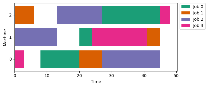
However, we can see that even for this simple problem, the solver could not find the optimal solution for the time-indexed model within the limit of 20 seconds.
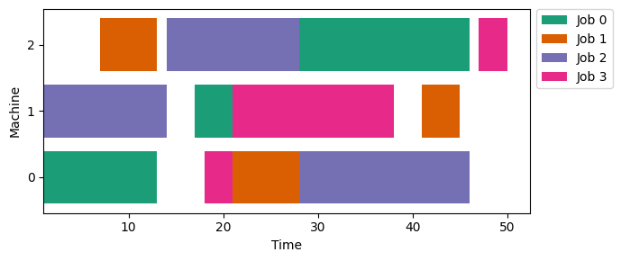
Amazing to see the difference in performance for two models with the same idea just by rearranging the mathematical equations.
By the way, those interested might find the complete code (plots included) in this repository.
Further reading
For larger instances, due to combinatorial aspects of this problem, even high-performance commercial solvers, such as Gurobi or Cplex, might face difficulties to provide good quality solutions and prove optimality. In this context, metaheuristics can be an interesting alternative. I would suggest the interested reader to look for the papers “Parallel GRASP with path-relinking for job shop scheduling” (Aiex et al., 2003) and “An extended Akers graphical method with a biased random-key genetic algorithm for job-shop scheduling” (Gonçalves & Resende, 2014). I recently tried to implement simplified versions of these algorithms and had some interesting results, although pure Python implementation is still time-expensive. You can find them in this repository.
Conclusions
In this article, two different mixed-integer programming approaches for the job-shop scheduling problem (JSSP) were implemented and solved using the Python library pyomo and the open-source solver CBC. The disjunctive model proved to be a better alternative for the original JSSP, although more complex real-world models might share similarities with the time-indexed formulation for incorporating additional rules. The complete code used in these examples is available for further use.
References
Aiex, R. M., Binato, S., & Resende, M. G. (2003). Parallel GRASP with path-relinking for job shop scheduling. Parallel Computing, 29(4), 393–430.
Bynum, M. L. et al., 2021. Pyomo-optimization modeling in python. Springer.
Gonçalves, J. F., & Resende, M. G. (2014). An extended Akers graphical method with a biased random‐key genetic algorithm for job‐shop scheduling. International Transactions in Operational Research, 21(2), 215–246.
Kondili, E., & Sargent, R. W. H. (1988). A general algorithm for scheduling batch operations (pp. 62–75). Department of Chemical Engineering, Imperial College.
Ku, W. Y., & Beck, J. C. (2016). Mixed integer programming models for job shop scheduling: A computational analysis. Computers & Operations Research, 73, 165–173.
Manne, A. S. (1960). On the job-shop scheduling problem. Operations research, 8(2), 219–223.
Wagner, H. M. (1959). An integer linear‐programming model for machine scheduling. Naval research logistics quarterly, 6(2), 131–140.
The Job-Shop Scheduling Problem: Mixed-Integer Programming Models was originally published in Towards Data Science on Medium, where people are continuing the conversation by highlighting and responding to this story.
...