

 800+ IT
News
als RSS Feed abonnieren
800+ IT
News
als RSS Feed abonnieren📚 Simulating Physical Systems with Python
💡 Newskategorie: AI Nachrichten
🔗 Quelle: towardsdatascience.com
A Must-Have Skill for any Engineer or Scientist

The ability to simulate the behavior of a physical system has incredible utility in nearly all fields of science and engineering. Simulations allow us to understand the time evolution of a system, and they do so in a manner that cannot typically be paralleled (even by physical testing). Whereas physical testing can be time consuming, expensive, and possibly dangerous, simulations are fast, cheap, and don’t pose any risks of equipment damage or bodily injury. Experiments are also limited in the sense that they only provide you access to data that you can actually measure — unmeasured system states will either not be available, or will have to be estimated in post processing. Simulations on the other hand, act as windows that allow us peer into the entire internal state of a system. This ability to essentially look into the inner workings of a system can provide invaluable design insight in engineering applications.
The intent of this article is to provide a quick primer on how to get started with simulating physical systems in the Python programming language. To accomplish this, we’re going to walk through a comprehensive example of how to simulate a bouncing ball. I’ve specifically chosen this system because it’s intuitive and not too difficult, but still has some nuances that make simulating it a little more interesting than other simple examples you’ll find on the internet (the equations that govern the motion of the ball change depending on whether the ball is in the air, or in contact with the ground). Along the way, we’ll look at how to convert a mathematical model to the correct format needed for simulating, show how we can leverage pre-existing code libraries (solve_ivp from SciPy) to make our lives easier, and give rationale as to why we’re structuring our code the way we are. By the end of this article, we’ll not only have a working simulation of a bouncing ball (like the animation shown below) but a foundational knowledge that can be extended to simulate any kind of physical system.
The Maths
Almost all systems in the physical world can be modeled by differential equations. These equations arise naturally from the physical laws that govern the world around us. Take Newton’s second law for example:

Newton’s second law tells us that the second derivative of the position of a mass is proportional to the net force applied to that mass. And thus we get a differential equation — an equation, that when solved gives us a function. For our problem, given a forcing function f(t), solving the above differential equation gives us the position of the mass as a function of time, x(t).
Great, so how do we go about solving the above differential equation? Unfortunately, there’s no general analytic method that we can use, as the solution is completely dependent on the forcing function, f(t). Depending on the form of the forcing function, solving the above differential equation can either be incredibly easy, or intractably difficult. This is where simulation comes into the picture. Simulation gives us a general purpose method for solving arbitrarily difficult differential equations!
So how does simulation work? When I say simulation, I’m essentially just referring to the numerical integration of a differential equation. There are ton’s of algorithms that exist to do this, such as the incredibly simple, but sometimes inaccurate Euler’s method, or Runge-Kutta methods, which are incredibly popular and more accurate. Rather than diving into the specifics of how these algorithms work, we’re going to treat them as a black box and leverage pre-existing code libraries that already have them implemented. To do this, however, we need to formulate our problem in a manner that fit’s the format required by these algorithms.
Numerical integration algorithms typically require that we input our equations as a system of first order differential equations. The general format for this is shown below, where t is time and x is a vector of system variables/states.

Looking at the above equation, we can see that the rate of change of each state in our system is influenced by the current state of the system and the instantaneous time. More often than not though, our system’s differential equations won’t naturally fall into this form (Newton’s second law, for example, is not a first order differential equation). Instead, we will typically have to massage our system’s equations into this format using some algebraic manipulation. This is all pretty abstract right now, so in the next section we’ll solidify the concept by applying the methodology to our bouncing ball problem.
Bouncing Ball Problem
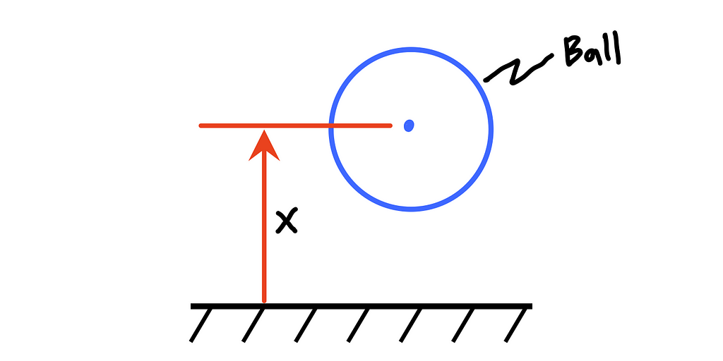
For the case of a bouncing ball, we have two scenarios that we need to consider: 1) when the ball is in the air, and 2) when the ball is in contact with the ground. In both cases, we’ll use Newton’s second law, but the form that the equations take will change a bit because the external forces applied to the ball change. To formulate the equations of motion, we will use the coordinate system shown below, where x represents the height of the center of the ball from the ground.
Step 1: Derive the System’s Equations
Case 1) the ball is in the air: When the ball is in the air the only force acting on the ball is gravity, and thus we get the following:

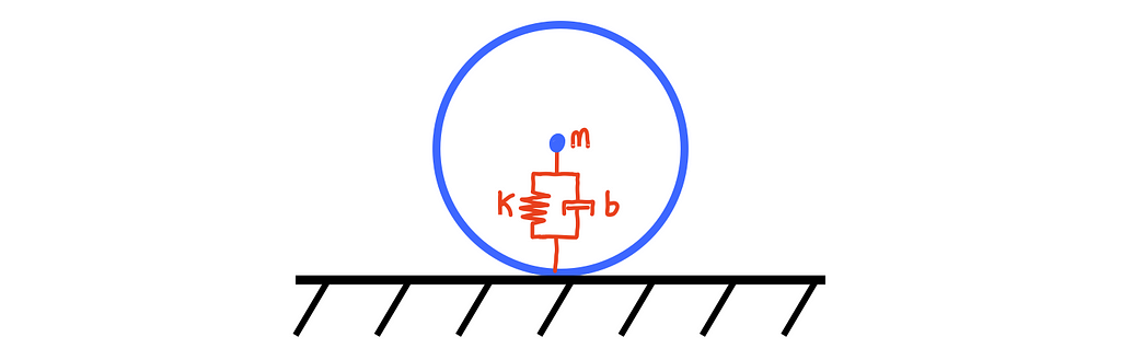
Case 2) the ball is in contact with the ground: Many different contact models exist for colliding objects, but for this example, we’re going to assume that the ball acts like a mass-spring-damper system. That is, we’ll assume that all of mass of the ball is concentrated at the center of the ball and the ball compresses on impact with some amount of stiffness (k) and damping (b). This is depicted below:
Drawing the free body diagram for the ball in contact with the ground, we get the following:
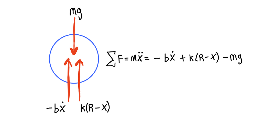
The three forces acting on the ball are gravity, damping, and the spring force produced within the ball. Note that the amount the spring (ball) compresses is equal to the radius of the ball (R), minus the position of the ball (x). Rearranging the equation a bit, we get the well known mass-spring-damper differential equation with forcing.

Step 2: Convert the Equations to the Correct Format for Simulation
We’ve derived a set of differential equations that govern the motion of the ball both in flight and in contact with the ground. Unfortunately, they’re not usable for simulation in their current form — we must convert them to a set of first order equations. To do this, we’ll introduce two new variables, x1 and x2, as follows:

Variables x1 and x2 are known as state variables and the vector containing them is called the state vector. The state vector, by definition, contains all of the information required to completely define the state of the system (in our case, the position and velocity of the ball). In general, if we have an nth order differential equation, we will have to introduce n new state variables (one for x and each of its derivatives, up to but not including the highest order derivative). We introduce two state variables in our example because we have a second order differential equation.
Differentiating the state vector yields:

Note that the derivative of x1 is, by definition, x2. I’ve purposely left the x-double-dot term as it is because it’s expression depends on whether the ball is in the air or in contact with the ground.
For the case of the ball being in flight, we have:

And for the case of the ball being in contact with the ground, we have:

Substituting the two x-double-dot expressions into the state derivative equation above yields the following two, vector-valued, state-derivative equations, applicable when the ball is in the air and in contact, respectively.


At this point we’ve successfully converted our higher-order differential equations into systems of first order equations and are ready to start coding up our simulation!
Step 3: The Code
To begin, we will import the necessary modules, as well as set some plotting settings to personal preference. The key line of code below is the from scipy.integrate import solve_ivp line, which imports the solver we’ll be using for our simulation (Note that ivp stands for “initial value problem” i.e. a differential equation with a given initial value).
import numpy as np
from scipy.integrate import solve_ivp
import matplotlib.pyplot as plt
import pandas as pd

#set default plotting settings to personal preference
font_settings = {'family':'Times New Roman', 'size':12}
line_settings = {'lw':2}
plt.rc('font', **font_settings)
plt.rc('lines', **line_settings)
We will organize our code by creating a BouncingBall class — a template for which is shown below with notes for what needs to be implemented in each method. We will populate each of these methods one-by-one
class BouncingBall():

    def __init__(self, m, k, b, ball_radius_cm):
        #TODO: initialize the physical properties of the ball
        pass

    def in_air(self,t,x):
        #TODO: compute the in-air physics of the ball (return the
        # rate of change of the ball's current state)
        pass

    def in_contact(self,t,x):
        #TODO: compute the in-contact physics of the ball (return the
        # rate of change of the ball's current state)
        pass

    def simulate(self, t_span, x0, max_step=0.01):
        #TODO: use the two physics models (`in_air` and `in_contact`) to
        # actually simulate the trajectory of the ball given a desired time
        # span and initial conditions. Must switch between the two physics
        # models at the appropriate times
        pass
First, we will look at the __init__ method. As can be seen in the code below, the __init__ method simply takes in and stores the various physical parameters of the ball. If no value is given for gravity, the standard value of 9.81 m/s² is assigned by default.
    def __init__(self, m, k, b, ball_radius_cm, gravity=None):
        """
        Parameters
        ----------
        m : float
            ball mass in kg
        k : float
            ball stiffness in N/m
        c : float
            ball viscous damping coef. in N/(m/s)
        ball_radius_cm : float
            ball radius in centimeters
        gravity : float, optional
            acceleration of gravity in m/s^2. Defaults to 9.81 m/s^2
            if None given.
        """

        self.r = ball_radius_cm/100 #radius in meters
        self.m = m
        self.k = k
        self.b = b

        if gravity is None:
            self.g = 9.81 #m/s^2
        else:
            self.g = gravity #m/s^2
Next, we’ll populate the two physics methods (in_air and in_contact). Both of the methods (below) take in an array x and the current time t, unpack the x array into x1 and x2 and then compute and return the state derivative vector according to the equations we derived in Step 2.
    def in_air(self,t,x):
        """computes the ball's state derivatives while in air

        Parameters
        ----------
        t : float
            simulation time
        x : array-like
            vector containing the ball's state variables (height and velocity)

        Returns
        -------
        list
            vector containing the ball's state derivatives
        """

        x1, x2 = x #unpack the current state of the ball
        return [x2, -self.g]

    def in_contact(self,t,x):
        """computes the ball's state derivatives while in contact with the ground

        Parameters
        ----------
        t : float
            simulation time
        x : array-like
            vector containing the ball's state variables (height and velocity)

        Returns
        -------
        list
            vector containing the ball's state derivatives
        """

        x1, x2 = x #unpack the current state of the ball
        x1_dot = x2
        x2_dot = -(self.b/self.m)*x2 + (self.k/self.m)*(self.r - x1) - self.g
        return [x1_dot, x2_dot]
Finally, we can populate the simulate method of the bouncing ball class, which will actually perform all of the interesting work. This method needs to integrate the physics of the ball forward in time, being sure to switch between the in-air and in-contact physics model when appropriate. Note that with how we’ve defined our coordinate system, the ball will be in contact with the ground when the position of the ball (x) is less than the ball’s radius (R).
The simplest way to switch between the two physics models would be to define an intermediate method that switches between the two previously defined methods depending on the position of the ball. It could look something like the following:
def ball_physics(self, t, x):

    #unpack ball's height and velocity
    x1, x2 = x

    #check if ball's center height is less than ball's radius
    if x1 <= self.R:
        #compute in-contact physics (state derivative)
        return self.in_contact(t,x)
    else:
        #compute in-air physics (state derivative)
        return self.in_air(t,x)
We would then pass this single function to the numerical integrator solve_ivp and solve the system forward in time. There is one major issue with this approach though, and that is that it will not precisely capture the moments of contact when the physics model needs to change. The figure below clarifies.
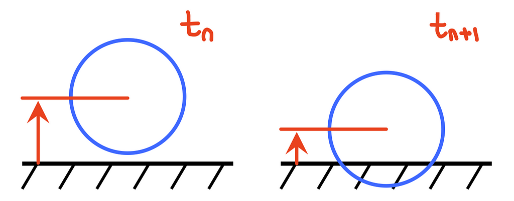
At time step tn, the ball is just above the ground and moving downward. The numerical integrator will then integrate the ball’s trajectory forward in time to time step tn+1. Note that the time difference between tn and tn+1 depends on the type of solver being used (fixed or variable step) and the corresponding error tolerance settings. Regardless, at time tn+1, the physics model will change to the in-contact model, but there’s an issue — the ball is already well into contact with the ground before the model changes. We don’t want the physics model to change any time the ball’s position (x) is less than the ball’s radius (R), we want the physics model to change at the EXACT instant the ball comes into contact, i.e. when the ball’s position equals the ball’s radius (x = R). To do this, we need another approach, we must use “events”.
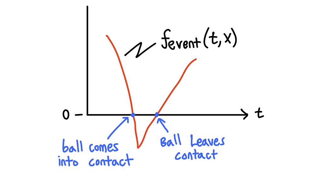
Intuitively, “events” are exactly as they sound — a point in time of particular interest, where “something” happens. In our case, we will be trying to capture two different events 1) the instant the ball comes into contact with the ground and 2) the instant the ball leaves contact with the ground. The way we mathematically describe an event is by defining a function that equals zero when an event occurs (for those familiar with Simulink, this is the same concept as “zero-crossings”). For our bouncing ball problem, this is simply the difference between the ball’s position and radius, as follows:

When the above function is zero, the height of the ball equals the ball’s radius, and thus we have a contact event. Furthermore, we can see looking at the figure below that when the event function crosses zero in the negative direction (going from positive to negative), this signals that the ball is coming into contact with the ground. Likewise, when the event function crosses zero in the positive direction (going from negative to positive), this signals that the ball is leaving contact with the ground.
Great, but how do we use this? Luckily for us, the notion of an event is already implemented in the solver we want to use (solve_ivp)— we just have to use it correctly! Looking at the SciPy documentation for solve_ivp, we see that there’s an optional argument events that takes in an arbitrary object. This object must be callable, meaning that we can call it like a function (this is exactly the event function that we defined above). The object also has additional attributes terminal and direction. If the terminal attribute is set to True, the simulation will terminate when an event occurs. The direction attribute is an additional flag that can be set to determine which of the zero-crossing directions to pay attention to. For example, if direction=-1, only the negative direction crossing (e.g. ball coming into contact with the ground) will count as an event, the positive crossing will just be ignored.
We can construct a class called ContactEvent that does exactly what the documentation is requiring. Looking at the code below, we see that the class takes in the ball’s radius and uses it for the event function, which is defined in the __call__ method (we have to implement it in the __call__ method because solve_ivp requires that the event object is callable). The ContactEvent class also contains the attributes direction and terminal. Note that terminal is set to True meaning the simulation will stop when an event occurs. The direction attribute is set at instantiation as it depends on the type of event we are trying to capture.
class ContactEvent():
    """Callable class that returns zero when the ball engages/disengages
    contact with the ground.
    """

    def __init__(self, r, direction=0):
        """
        Parameters
        ----------
        r : float
            Radius of the ball in meters
        direction : int, optional
            Direction of a zero crossing to trigger the contact event.
            Negative for the ball coming into contact with the ground.
            Positive for the ball leaving contact with the ground, by default 0
        """

        self.r = r
        self.direction = direction
        self.terminal = True #terminal is True so that simulation will end on contact event

    def __call__(self,t,x):
        """Computes the height of the ball above being in contact

        Notes
        -----
        The ball will engage/disengage contact when the height of the center
        of the ball equals the radius of the ball.

        Parameters
        ----------
        t : float
            time in the simulation
        x : array-like
            vector of ball's state variables (height and velocity)

        Returns
        -------
        float
            height above being in contact
        """
        #unpack height and velocity of ball
        x1, x2 = x
        return x1 - self.r
To use the ContactEvent class, we will create two ContactEvent objects (one for the ball coming into contact and one for the ball leaving contact) and store them in the BouncingBall object. To do this, we’ll add two more lines of code to the __init__ method as follows:
def __init__(self, m, k, b, ball_radius_cm, gravity=None):
        """
        Parameters
        ----------
        m : float
            ball mass in kg
        k : float
            ball stiffness in N/m
        c : float
            ball viscous damping coef. in N/(m/s)
        ball_radius_cm : float
            ball radius in centimeters
        gravity : float, optional
            acceleration of gravity in m/s^2. Defaults to 9.81 m/s^2
            if None given.
        """

        self.r = ball_radius_cm/100 #radius in meters
        self.m = m
        self.k = k
        self.b = b

        if gravity is None:
            self.g = 9.81 #m/s^2
        else:
            self.g = gravity #m/s^2


        # create event functions for the ball engaging and disengaging contact
        # note that when coming into contact with the ground, the direction of the
        # zero crossing will be negative (height abve the ground is transitioning
        # to negative) whereas when the ball leaves the ground the zero crossing
        # will be positive (height above the ground is transitioning from negative
        # to positive)
        self.hitting_ground = ContactEvent(self.r, direction=-1)
        self.leaving_ground = ContactEvent(self.r, direction=1)
With our contact event functions defined, we can finally look at the simulate method code (below).
def simulate(self, t_span, x0, max_step=0.01):
        """Simulates the time evolution of the ball bouncing

        Parameters
        ----------
        t_span : two element tuple/list
            starting and stopping time of the simulation, e.g. (0,10)
        x0 : array-like
            initial conditions of ball (height and velocity in m and m/s)
        max_step : float, optional
            max step size in simulation, by default 0.01

        Returns
        -------
        tuple
            tuple containing the time vector and height of the ball
        """

        #check the initial height of the ball to determine if it's starting in the air
        in_air = x0[0] > self.r
        #extract out initial starting and stopping times
        t_start, t_stop = t_span

        #create lists with initial conditions that we can append the piecewise solutions to
        t_lst = [t_start]
        x_lst = [x0[0]]

        #loop until we reach the desired stopping time
        while t_start < t_stop:

            """
            Here we simulate the ball forward in time using either the air
            or contact model. Each of these subroutines will terminate when
            either 1) the final desired simulation stop time is reached,
            or 2) when a contact event is triggered. At a high level, we are
            simulating our system forward in time using the relevant physics
            model (that depends on the state of the system). The simulation
            will alternate between the "in_air" model and "in_contact" model
            switching between the two each time a contact event is triggered
            """

            if in_air:
                sol = solve_ivp(self.in_air, [t_start, t_stop], x0,
                                events=[self.hitting_ground], max_step=max_step)

            else:
                sol = solve_ivp(self.in_contact, [t_start, t_stop], x0,
                                events=[self.leaving_ground], max_step=max_step)

            # append solution and time array to list of solutions.
            # Note that the starting time of each solution
            # is the stopping time of the previous solution.
            # To avoid having duplicate time points, we will not include the first
            #data point of each simulation. This is also why we created our
            # solution lists above with the initial conditions already in them
            t_lst.append(sol.t[1::])
            x_lst.append(sol.y[0,1::])

            #set the starting time and initial conditions to the stopping
            #time and end condtions of the previous loop
            t_start = sol.t[-1]
            x0 = sol.y[:,-1].flatten()

            #if we haven't reached the stopping time yet in the current
            #loop, we must be switching between being in the air and
            #being in contact
            if t_start < t_stop:
                in_air = not in_air

        #concatenate all of the solutions into a single numpy array
        t = np.hstack(t_lst)
        x = np.hstack(x_lst)

        return t,x
As can be seen in the code above, the simulate method takes in the initial conditions and a time span that we would wish to solve for. It first check’s if the ball is starting in the air, or in contact with the ground to determine which physics model to use initially. The code that follows then works as follows:
- Create two lists (t_lst and x_lst) that we can keep appending the piecewise simulation solutions to.
- Simulate the ball forward in time, passing the appropriate physics model and event object to solve_ivp (Note thatsolve_ivp takes in a function that returns the state derivative vector (as discussed in step 2), initial conditions, and a time span to solve for). Simulate forward in time until a contact event happens, at which point the simulation stops. Append the simulation time and solutions to t_lst and x_lst respectively.
- Switch the physics model (every event signals the switching of the physics model) and reset the initial conditions and starting time to equal the final conditions and time of the previous solve.
- Repeat 2 and 3 until the desired final simulation time is reached.
- Concatenate all of the time and solution vectors into single arrays and return the solution.
The complete BouncingBall class is shown below.
class BouncingBall():
    """Class to simulate a bouncing ball

    Methods
    -------
    in_air(t, x) : Computes the ball's state derivatives while in air

    in_contact(t, x) : Computes the ball's state derivatives while in contact

    simulate(t_span, x0, max_step) : Simulates the ball bouncing
    """

    def __init__(self, m, k, b, ball_radius_cm, gravity=None):
        """
        Parameters
        ----------
        m : float
            ball mass in kg
        k : float
            ball stiffness in N/m
        c : float
            ball viscous damping coef. in N/(m/s)
        ball_radius_cm : float
            ball radius in centimeters
        gravity : float, optional
            acceleration of gravity in m/s^2. Defaults to 9.81 m/s^2
            if None given.
        """

        self.r = ball_radius_cm/100 #radius in meters
        self.m = m
        self.k = k
        self.b = b

        if gravity is None:
            self.g = 9.81 #m/s^2
        else:
            self.g = gravity #m/s^2


        # create event functions for the ball engaging and disengaging contact
        # note that when coming into contact with the ground, the direction of the
        # zero crossing will be negative (height abve the ground is transitioning
        # to negative) whereas when the ball leaves the ground the zero crossing
        # will be positive (height above the ground is transitioning from negative
        # to positive)
        self.hitting_ground = ContactEvent(self.r, direction=-1)
        self.leaving_ground = ContactEvent(self.r, direction=1)

    def in_air(self,t,x):
        """computes the ball's state derivatives while in air

        Parameters
        ----------
        t : float
            simulation time
        x : array-like
            vector containing the ball's state variables (height and velocity)

        Returns
        -------
        list
            vector containing the ball's state derivatives
        """

        x1, x2 = x #unpack the current state of the ball
        return [x2, -self.g]

    def in_contact(self,t,x):
        """computes the ball's state derivatives while in contact with the ground

        Parameters
        ----------
        t : float
            simulation time
        x : array-like
            vector containing the ball's state variables (height and velocity)

        Returns
        -------
        list
            vector containing the ball's state derivatives
        """

        x1, x2 = x #unpack the current state of the ball
        x1_dot = x2
        x2_dot = -(self.b/self.m)*x2 + (self.k/self.m)*(self.r - x1) - self.g
        return [x1_dot, x2_dot]

    def simulate(self, t_span, x0, max_step=0.01):
        """Simulates the time evolution of the ball bouncing

        Parameters
        ----------
        t_span : two element tuple/list
            starting and stopping time of the simulation, e.g. (0,10)
        x0 : array-like
            initial conditions of ball (height and velocity in m and m/s)
        max_step : float, optional
            max step size in simulation, by default 0.01

        Returns
        -------
        tuple
            tuple containing the time vector and height of the ball
        """

        #check the initial height of the ball to determine if it's starting in the air
        in_air = x0[0] > self.r
        #extract out initial starting and stopping times
        t_start, t_stop = t_span

        #create lists with initial conditions that we can append the piecewise solutions to
        t_lst = [t_start]
        x_lst = [x0[0]]

        #loop until we reach the desired stopping time
        while t_start < t_stop:

            """
            Here we simulate the ball forward in time using either the air
            or contact model. Each of these subroutines will terminate when
            either 1) the final desired simulation stop time is reached,
            or 2) when a contact event is triggered. At a high level, we are
            simulating our system forward in time using the relevant physics
            model (that depends on the state of the system). The simulation
            will alternate between the "in_air" model and "in_contact" model
            switching between the two each time a contact event is triggered
            """

            if in_air:
                sol = solve_ivp(self.in_air, [t_start, t_stop], x0,
                                events=[self.hitting_ground], max_step=max_step)

            else:
                sol = solve_ivp(self.in_contact, [t_start, t_stop], x0,
                                events=[self.leaving_ground], max_step=max_step)

            # append solution and time array to list of solutions.
            # Note that the starting time of each solution
            # is the stopping time of the previous solution.
            # To avoid having duplicate time points, we will not include the first
            #data point of each simulation. This is also why we created our
            # solution lists above with the initial conditions already in them
            t_lst.append(sol.t[1::])
            x_lst.append(sol.y[0,1::])

            #set the starting time and initial conditions to the stopping
            #time and end condtions of the previous loop
            t_start = sol.t[-1]
            x0 = sol.y[:,-1].flatten()

            #if we haven't reached the stopping time yet in the current
            #loop, we must be switching between being in the air and
            #being in contact
            if t_start < t_stop:
                in_air = not in_air

        #concatenate all of the solutions into a single numpy array
        t = np.hstack(t_lst)
        x = np.hstack(x_lst)

        return t,x
At this point all of the hard work is done and we’re ready to run a simulation! We can do so using the following few lines of code, which create a BouncingBall object, simulate the ball bouncing for eight seconds after being dropped from 2 meters, and then plot the trajectory.
b = BouncingBall(m=1, k=10e3, c=10, ball_radius_cm=6)

t,x = b.simulate([0,8], [2, 0])
df = pd.DataFrame({'time':t, 'x':x}).set_index('time')
df.to_csv('sim_data.csv')

fig, ax = plt.subplots()
ax.plot(t,x)
ax.set_xlabel('Time [s]')
ax.set_ylabel('Height [m]')

fig.savefig('bouncing_ball.png')
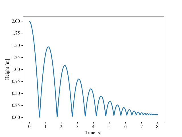
Pretty satisfying! If we wanted, we could even post-process the data to create an animation of the ball bouncing (like the one at the beginning of the post and repeated here).
Creating animations in matplotlib is beyond the scope of this article, but for those interested, the code to create the animation is included in this articles accompanying Github repository.
Conclusion
The ability to simulate a physical system can provide invaluable utility in nearly all fields of science and engineering. The highlighted example, though rather specific, covered a much more general workflow that can be extended to simulating any type of physical system. Regardless of the system, you will always have to determine the governing equations, convert them to a system of first order differential equations, and then pass the equations to a numerical integration routine of some sort. Of course, there are some nuances that couldn’t be discussed in this article — sometimes the system contains constraint equations and we get a set of differential algebraic equations (DAEs) instead of ordinary differential equations (ODEs). Or you may not be able to solve for your state vector derivative explicitly in terms of the systems states. Regardless, the content covered in this article still serves as a necessary foundation that must be mastered before moving onto more involved studies.
Feel free to leave any comments or questions you may have or connect with me on Linkedin — I’d be more than happy to clarify any points of uncertainty. Finally, I encourage you to play around with the code yourself (or even use it as a starting template for your own workflows ) — all code for this article can be found on my Github.
Nicholas Hemenway
- If you enjoyed this, please follow me on Medium
- Consider subscribing to email updates
- Interested in collaborating? Let’s connect on LinkedIn
Simulating Physical Systems with Python was originally published in Towards Data Science on Medium, where people are continuing the conversation by highlighting and responding to this story.
...