📚 Deriving a Score to Show Relative Socio-Economic Advantage and Disadvantage of a Geographic Area

Using Principal Component Analysis with Real-life data

Motivation

There exist publicly accessible data which describe the socio-economic characteristics of a geographic location. In Australia where I reside, the Government through the Australian Bureau of Statistics (ABS) collects and publishes individual and household data on a regular basis in respect of income, occupation, education, employment and housing at an area level. Some examples of the published data points include:

• Percentage of people on relatively high / low income
• Percentage of people classified as managers in their respective occupations
• Percentage of people with no formal educational attainment
• Percentage of people unemployed
• Percentage of properties with 4 or more bedrooms

Whilst these data points appear to focus heavily on individual people, it reflects people’s access to material and social resources, and their ability to participate in society in a particular geographic area, ultimately informing the socio-economic advantage and disadvantage of this area.

Given these data points, is there a way to derive a score which ranks geographic areas from the most to the least advantaged?

The Problem

The goal to derive a score may formulate this as a regression problem, where each data point or feature is used to predict a target variable, in this scenario, a numerical score. This requires the target variable to be available in some instances for training the predictive model.

However, as we don’t have a target variable to start with, we may need to approach this problem in another way. For instance, under the assumption that each geographic areas is different from a socio-economic standpoint, can we aim to understand which data points help explain the most variations, thereby deriving a score based on a numerical combination of these data points.

We can do exactly that using a technique called the Principal Component Analysis (PCA), and this article demonstrates how!

The Data

ABS publishes data points indicating the socio-economic characteristics of a geographic area in the “Data Download” section of this webpage, under the “Standardised Variable Proportions data cube”[1]. These data points are published at the Statistical Area 1 (SA1) level, which is a digital boundary segregating Australia into areas of population of approximately 200–800 people. This is a much more granular digital boundary compared to the Postcode (Zipcode) or the States digital boundary.

For the purpose of demonstration in this article, I’ll be deriving a socio-economic score based on 14 out of the 44 published data points provided in Table 1 of the data source above (I’ll explain why I select this subset later on). These are :

• INC_LOW: Percentage of people living in households with stated annual household equivalised income between $1 and $25,999 AUD
• INC_HIGH: Percentage of people with stated annual household equivalised income greater than $91,000 AUD
• UNEMPLOYED_IER: Percentage of people aged 15 years and over who are unemployed
• HIGHBED: Percentage of occupied private properties with four or more bedrooms
• HIGHMORTGAGE: Percentage of occupied private properties paying mortgage greater than $2,800 AUD per month
• LOWRENT: Percentage of occupied private properties paying rent less than $250 AUD per week
• OWNING: Percentage of occupied private properties without a mortgage
• MORTGAGE: Per cent of occupied private properties with a mortgage
• GROUP: Percentage of occupied private properties which are group occupied private properties (e.g. apartments or units)
• LONE: Percentage of occupied properties which are lone person occupied private properties
• OVERCROWD: Percentage of occupied private properties requiring one or more extra bedrooms (based on Canadian National Occupancy Standard)
• NOCAR: Percentage of occupied private properties with no cars
• ONEPARENT: Percentage of one parent families
• UNINCORP: Percentage of properties with at least one person who is a business owner

The Steps

In this section, I’ll be stepping through the Python code for deriving a socio-economic score for a SA1 region in Australia using PCA.

I’ll start by loading in the required Python packages and the data.

## Load the required Python packages

### For dataframe operations
import numpy as np
import pandas as pd

### For PCA
from sklearn.decomposition import PCA
from sklearn.preprocessing import StandardScaler

### For Visualization
import matplotlib.pyplot as plt
import seaborn as sns

### For Validation
from scipy.stats import pearsonr

## Load data

file1 = 'data/standardised_variables_seifa_2021.xlsx'

### Reading from Table 1, from row 5 onwards, for column A to AT
data1 = pd.read_excel(file1, sheet_name = 'Table 1', header = 5,
                      usecols = 'A:AT')

## Remove rows with missing value (113 out of 60k rows)

data1_dropna = data1.dropna()

An important cleaning step before performing PCA is to standardise each of the 14 data points (features) to a mean of 0 and standard deviation of 1. This is primarily to ensure the loadings assigned to each feature by PCA (think of them as indicators of how important a feature is) are comparable across features. Otherwise, more emphasis, or higher loading, may be given to a feature which is actually not significant or vice versa.

Note that the ABS data source quoted above already have the features standardised. That said, for an unstandardised data source:

## Standardise data for PCA

### Take all but the first column which is merely a location indicator
data_final = data1_dropna.iloc[:,1:]

### Perform standardisation of data
sc = StandardScaler()
sc.fit(data_final)

### Standardised data
data_final = sc.transform(data_final)

With the standardised data, PCA can be performed in just a few lines of code:

## Perform PCA

pca = PCA()
pca.fit_transform(data_final)

PCA aims to represent the underlying data by Principal Components (PC). The number of PCs provided in a PCA is equal to the number of standardised features in the data. In this instance, 14 PCs are returned.

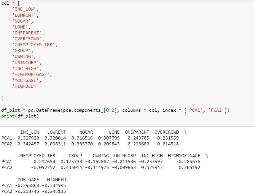
Each PC is a linear combination of all the standardised features, only differentiated by its respective loadings of the standardised feature. For example, the image below shows the loadings assigned to the first and second PCs (PC1 and PC2) by feature.

With 14 PCs, the code below provides a visualization of how much variation each PC explains:

## Create visualization for variations explained by each PC

exp_var_pca = pca.explained_variance_ratio_
plt.bar(range(1, len(exp_var_pca) + 1), exp_var_pca, alpha = 0.7,
            label = '% of Variation Explained',color = 'darkseagreen')
    
plt.ylabel('Explained Variation')
plt.xlabel('Principal Component')
plt.legend(loc = 'best')
plt.show()

As illustrated in the output visualization below, Principal Component 1 (PC1) accounts for the largest proportion of variance in the original dataset, with each following PC explaining less of the variance. To be specific, PC1 explains circa. 35% of the variation within the data.

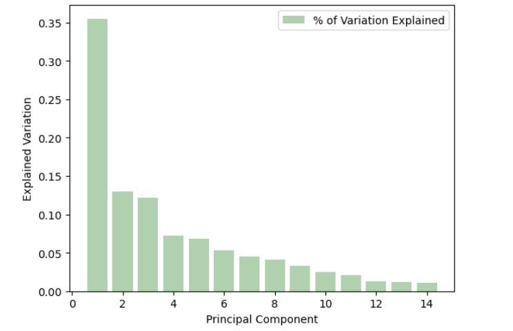
For the purpose of demonstration in this article, PC1 is chosen as the only PC for deriving the socio-economic score, for the following reasons:

• PC1 explains sufficiently large variation within the data on a relative basis.
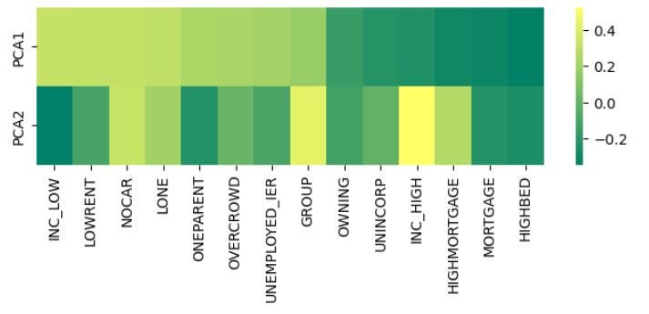
• Whilst choosing more PCs potentially allows for (marginally) more variation to be explained, it makes interpretation of the score difficult in the context of socio-economic advantage and disadvantage by a particular geographic area. For example, as shown in the image below, PC1 and PC2 may provide conflicting narratives as to how a particular feature (e.g. ‘INC_LOW’) influences the socio-economic variation of a geographic area.

## Show and compare loadings for PC1 and PC2

### Using df_plot dataframe per Image 1

sns.heatmap(df_plot, annot = False, fmt = ".1f", cmap = 'summer') 
plt.show()

To obtain a score for each SA1, we simply multiply the standardised portion of each feature by its PC1 loading. This can be achieved by:

## Obtain raw score based on PC1

### Perform sum product of standardised feature and PC1 loading
pca.fit_transform(data_final)

### Reverse the sign of the sum product above to make output more interpretable
pca_data_transformed = -1.0*pca.fit_transform(data_final)

### Convert to Pandas dataframe, and join raw score with SA1 column
pca1 = pd.DataFrame(pca_data_transformed[:,0], columns = ['Score_Raw'])
score_SA1 = pd.concat([data1_dropna['SA1_2021'].reset_index(drop = True), pca1]
                    , axis = 1)

### Inspect the raw score
score_SA1.head()

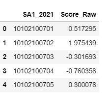
The higher the score, the more advantaged a SA1 is in terms its access to socio-economic resource.

The Validation

How do we know the score we derived above was even remotely correct?

For context, the ABS actually published a socio-economic score called the Index of Economic Resource (IER), defined on the ABS website as:

“The Index of Economic Resources (IER) focuses on the financial aspects of relative socio-economic advantage and disadvantage, by summarising variables related to income and housing. IER excludes education and occupation variables as they are not direct measures of economic resources. It also excludes assets such as savings or equities which, although relevant, cannot be included as they are not collected in the Census.”

Without disclosing the detailed steps, the ABS stated in their Technical Paper that the IER was derived using the same features (14) and methodology (PCA, PC1 only) as what we had performed above. That is, if we did derive the correct scores, they should be comparable against the IER scored published here (“Statistical Area Level 1, Indexes, SEIFA 2021.xlsx”, Table 4).

As the published score is standardised to a mean of 1,000 and standard deviation of 100, we start the validation by standardising the raw score the same:

## Standardise raw scores

score_SA1['IER_recreated'] = 
          (score_SA1['Score_Raw']/score_SA1['Score_Raw'].std())*100 + 1000

For comparison, we read in the published IER scores by SA1:

## Read in ABS published IER scores
## similarly to how we read in the standardised portion of the features

file2 = 'data/Statistical Area Level 1, Indexes, SEIFA 2021.xlsx'

data2 = pd.read_excel(file2, sheet_name = 'Table 4', header = 5,
                      usecols = 'A:C')

data2.rename(columns =  {'2021 Statistical Area Level 1 (SA1)': 'SA1_2021', 'Score': 'IER_2021'}, inplace = True)

col_select = ['SA1_2021', 'IER_2021']
data2 = data2[col_select]

ABS_IER_dropna = data2.dropna().reset_index(drop = True)

Validation 1— PC1 Loadings

Comparing the PC1 loading derived above against the PC1 loading published by the ABS suggests that

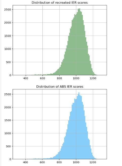
Validation 2— Distribution of Scores

The code below creates a histogram for both scores, whose shapes look to be almost identical.

## Check distribution of scores

score_SA1.hist(column = 'IER_recreated', bins = 100, color = 'darkseagreen')
plt.title('Distribution of recreated IER scores')

ABS_IER_dropna.hist(column = 'IER_2021', bins = 100, color = 'lightskyblue')
plt.title('Distribution of ABS IER scores')

plt.show()

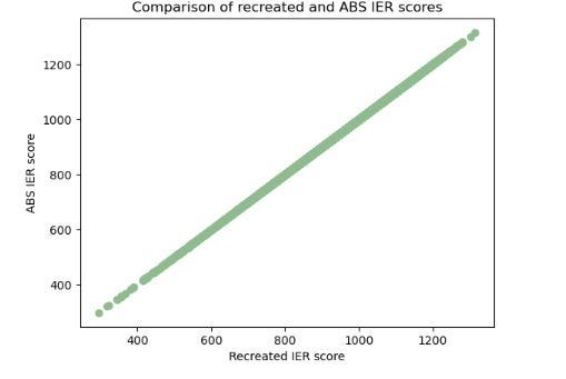
Validation 3— IER score by SA1

As the ultimate validation, let’s compare the IER scores by SA1:

## Join the two scores by SA1 for comparison
IER_join = pd.merge(ABS_IER_dropna, score_SA1, how = 'left', on = 'SA1_2021')

## Plot scores on x-y axis. 
## If scores are identical, it should show a straight line.

plt.scatter('IER_recreated', 'IER_2021', data = IER_join, color = 'darkseagreen')
plt.title('Comparison of recreated and ABS IER scores')
plt.xlabel('Recreated IER score')
plt.ylabel('ABS IER score')

plt.show()

A diagonal straight line as shown in the output image below supports that the two scores are largely identical.

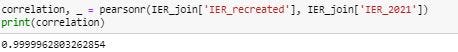
To add to this, the code below shows the two scores have a correlation close to 1:

Concluding Thought

The demonstration in this article effectively replicates how the ABS calibrates the IER, one of the four socio-economic indexes it publishes, which can be used to rank the socio-economic status of a geographic area.

Taking a step back, what we’ve achieved in essence is a reduction in dimension of the data from 14 to 1, losing some information conveyed by the data.

Dimensionality reduction technique such as the PCA is also commonly seen in helping to reduce high-dimension space such as text embeddings to 2–3 (visualizable) Principal Components.

Reference

[1] Australian Bureau of Statistics (2021), Socio-Economic Indexes for Areas (SEIFA), ABS Website, accessed 29 December 2023 (Creative Common Licence)

As I ride the AI/ML wave, I enjoy writing and sharing step-by-step guides and how-to tutorials in a comprehensive language with ready-to-run codes. If you would like to access all my articles (and articles from other practitioners/writers on Medium), you can sign up using the link here!

Deriving a Score to Show Relative Socio-Economic Advantage and Disadvantage of a Geographic Area was originally published in Towards Data Science on Medium, where people are continuing the conversation by highlighting and responding to this story.