📚 Mastering K-Means Clustering

Implement the K-Means algorithm from scratch with this step-by-step Python tutorial

In this article, I show how I’d learn the K-Means algorithm if I’d started today. We’ll start with the fundamental concepts and implement a Python class that performs clustering tasks using nothing more than the Numpy package.

Whether you are a machine learning beginner trying to build a solid understanding of the concepts or a practitioner interested in creating custom machine learning applications and needs to understand how the algorithms work under the hood, that article is for you.

Table of contents

1. Introduction
2. What Does the K-Means algorithm do?
3. Implementation in Python
4. Evaluation and Interpretation
5. Conclusions and Next Steps

1. Introduction

Most of the machine learning algorithms widely used, such as Linear Regression, Logistic Regression, Decision Trees, and others are useful for making predictions from labeled data, that is, each input comprises feature values with a label value associated. That is what is called Supervised Learning.

However, often we have to deal with large sets of data with no label associated. Imagine a business that needs to understand the different groups of customers based on purchasing behavior, demographics, address, and other information, thus it can offer better services, products, and promotions.

These types of problems can be addressed with the use of Unsupervised Learning techniques. The K-Means algorithm is a widely used unsupervised learning algorithm in Machine Learning. Its simple and elegant approach makes it possible to separate a dataset into a desired number of K distinct clusters, thus allowing one to learn patterns from unlabelled data.

2. What Does the K-Means algorithm do?

As said earlier, the K-Means algorithm seeks to partition data points into a given number of clusters. The points within each cluster are similar, while points in different clusters have considerable differences.

Having said that, one question arises: how do we define similarity or difference? In K-Means clustering, the Euclidean distance is the most common metric for measuring similarity.

In the figure below, we can clearly see 3 different groups. Hence, we could determine the centers of each group and each point would be associated with the closest center.

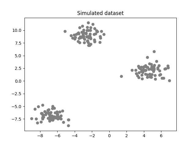
By doing that, mathematically speaking, the idea is to minimize the within-cluster variance, the measurement of similarity between each point and its closest center.

Performing the task in the example above was straightforward because the data was two-dimensional and the groups were clearly distinct. However, as the number of dimensions increases and different values of K are considered, we need an algorithm to handle the complexity.

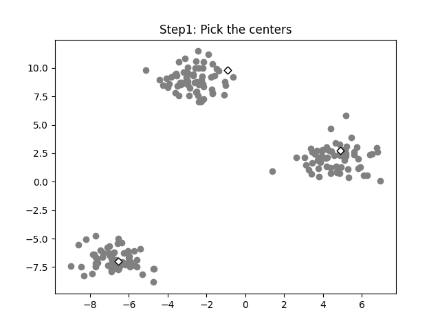
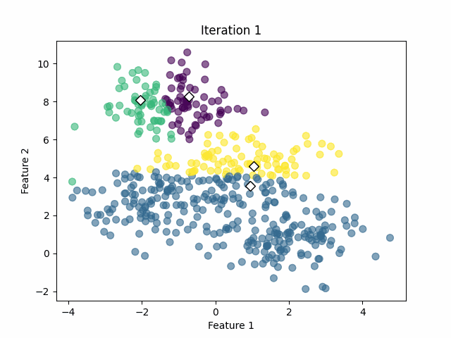
Step 1: Pick the initial centers (randomly)

We need to seed the algorithm with initial center vectors that can be chosen randomly from the data or generate random vectors with the same dimensions as the original data. See the white diamonds in the image below.

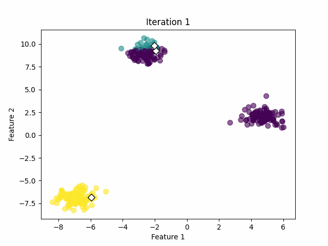
Step 2: Find the distances of each point to the centers

Now, we'll calculate the distance of each data point to the K centers. Then we associate each point with the center closest to that point.

Given a dataset with N entries and M features, the distances to the centers c can be given by the following equation:

where:

k varies from 1 to K;

D is the distance of a point n to the k center;

x is the point vector;

c is the center vector.

Hence, for each data point n we'll have K distances, then we have to label the vector to the center with the smallest distance:

Where D is a vector with K distances.

Step 3: Find the K centroids and iterate

For each of the K clusters, recalculate the centroid. The new centroid is the mean of all data points assigned to that cluster. Then update the positions of the centroids to the newly calculated.

Check if the centroids have changed significantly from the previous iteration. This can be done by comparing the positions of the centroids in the current iteration with those in the last iteration.

If the centroids have changed significantly, go back to Step 2. If not, the algorithm has converged and the process stops. See the image below.

3. Implementation in Python

Now that we know the fundamental concepts of the K-Means algorithm, it's time to implement a Python class. The packages used were Numpy for mathematical calculations, Matplotlib for visualization, and the Make_blobs package from Sklearn for simulated data.

# import required packages
import numpy as np
import matplotlib.pyplot as plt
from sklearn.datasets import make_blobs

The class will have the following methods:

• Init method

A constructor method to initialize the basic parameters of the algorithm: the value k of clusters, the maximum number of iterations max_iter, and the tolerance tol value to interrupt the optimization when there is no significant improvement.

• Helper functions

These methods aim to assist the optimization process during training, such as calculating the Euclidean distance, randomly choosing the initial centroids, assigning the closest centroid to each point, updating the centroids’ values, and verifying whether the optimization converged.

• Fit and predict method

As mentioned earlier, the K-Means algorithm is an unsupervised learning technique, meaning it does not require labeled data during the training process. That way, it's necessary a single method to fit the data and predict to which cluster each data point belongs.

• Total error method

A method to evaluate the quality of the optimization by calculating the total squared error of the optimization. That will be explored in the next section.

Here it goes the full code:

class Kmeans:
    
    # construct method for hyperparameter initialization
    def __init__(self, k=3, max_iter=100, tol=1e-06):
        self.k = k
        self.max_iter = max_iter
        self.tol = tol
  
    # randomly picks the initial centroids from the input data
    def pick_centers(self, X):
        centers_idxs = np.random.choice(self.n_samples, self.k)
        return X[centers_idxs]
    
    # finds the closest centroid for each data point
    def get_closest_centroid(self, x, centroids):
        distances = [euclidean_distance(x, centroid) for centroid in centroids]
        return np.argmin(distances)
    
    # creates a list with lists containing the idxs of each cluster
    def create_clusters(self, centroids, X):
        clusters = [[] for _ in range(self.k)]
        labels = np.empty(self.n_samples)
        for i, x in enumerate(X):
            centroid_idx = self.get_closest_centroid(x, centroids)
            clusters[centroid_idx].append(i)
            labels[i] = centroid_idx

        return clusters, labels
    
    # calculates the centroids for each cluster using the mean value 
    def compute_centroids(self, clusters, X):
        centroids = np.empty((self.k, self.n_features))
        for i, cluster in enumerate(clusters):
            centroids[i] = np.mean(X[cluster], axis=0)

        return centroids
    
    # helper function to verify if the centroids changed significantly
    def is_converged(self, old_centroids, new_centroids):
        distances = [euclidean_distance(old_centroids[i], new_centroids[i]) for i in range(self.k)]
        return (sum(distances) < self.tol)


    # method to train the data, find the optimized centroids and label each data point according to its cluster
    def fit_predict(self, X):
        self.n_samples, self.n_features = X.shape
        self.centroids = self.pick_centers(X)

        for i in range(self.max_iter):
            self.clusters, self.labels = self.create_clusters(self.centroids, X)
            new_centroids = self.compute_centroids(self.clusters, X)
            if self.is_converged(self.centroids, new_centroids):
                break
            self.centroids = new_centroids

    
    # method for evaluating the intracluster variance of the optimization
    def clustering_errors(self, X):
        cluster_values = [X[cluster] for cluster in self.clusters]
        squared_distances = []
        # calculation of total squared Euclidean distance
        for i, cluster_array in enumerate(cluster_values):
            squared_distances.append(np.sum((cluster_array - self.centroids[i])**2))

        total_error = np.sum(squared_distances)
        return total_error

4. Evaluation and Interpretation

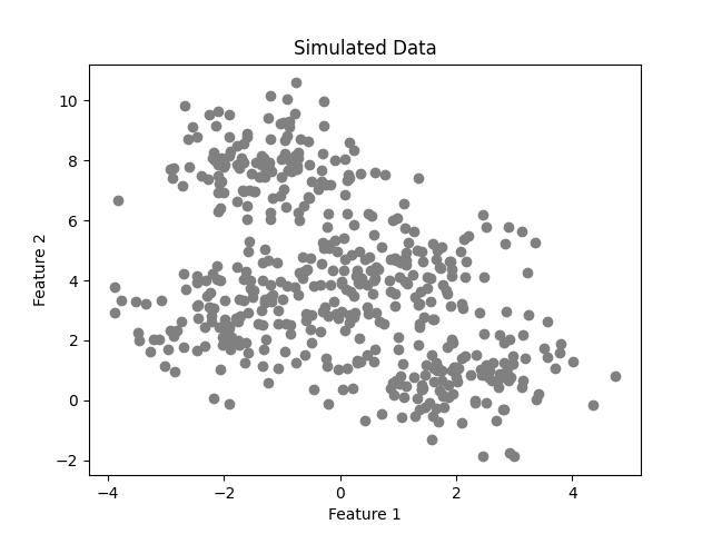
Now we'll use the K-Means class to perform the clustering of simulated data. To do that, it'll be used the make_blobs package from the Sklearn library. The data consists of 500 two-dimensional points with 4 fixed centers.

# create simulated data for examples
X, _ = make_blobs(n_samples=500, n_features=2, centers=4, 
                  shuffle=False, random_state=0)

After performing the training using four clusters, we achieve the following result.

model = Kmeans(k=4)
model.fit_predict(X)
labels = model.labels
centroids =model.centroids
plot_clusters(X, labels, centroids)

In that case, the algorithm was capable of calculating the clusters successfully with 18 iterations. However, we must keep in mind that we already know the optimal number of clusters from the simulated data. In real-world applications, we often don't know that value.

As said earlier, the K-Means algorithm aims to make the within-cluster variance as small as possible. The metric used to calculate that variance is the total squared Euclidean distance given by:

where:

p is the number of data points in a cluster;

c_i is the centroid vector of a cluster;

K is the number of clusters.

In words, the formula above adds up the distances of the data points to the nearest centroid. The error decreases as the number K increases.

In the extreme case of K =N, you have one cluster for each data point and this error will be zero.

Willmott, Paul (2019).

If we plot the error against the number of clusters and look at where the graph "bends", we'll be able to find the optimal number of clusters.

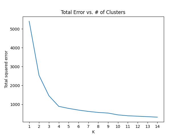
As we can see, the plot has an "elbow shape" and it bends at K = 4, meaning that for greater values of K, the decrease in the total error will be less significant.

5. Conclusions and Next Steps

In this article, we covered the fundamental concepts behind the K-Means algorithm, its uses, and applications. Also, using these concepts, we were able to implement a Python class from scratch that performed the clustering of simulated data and how to find the optimal value for K using a scree plot.

However, since we are dealing with an unsupervised technique, there is one additional step. The algorithm can successfully assign a label to the clusters, but the meaning of each label is a task that the data scientist or machine learning engineer will have to do by analyzing the data of each cluster.

In addition, I'll leave some points for further exploration:

• Our simulated data used two-dimensional points. Try to use the algorithm for other datasets and find the optimal values for K.
• There are other unsupervised learning algorithms widely used such as Hierarchical Clustering.
• Depending on the domain of the problem, it may be necessary to use other error metrics such as Manhattan distance and cosine similarity. Try to investigate them.

Complete code available here:

ML-and-Ai-from-scratch/K-Means at main · Marcussena/ML-and-Ai-from-scratch

Please feel free to use and improve the code, comment, make suggestions, and connect with me on LinkedIn, X, and Github.

References

[1] Sebastian Raschka (2015), Python Machine Learning.

[2] Willmott, Paul. (2019). Machine Learning: An Applied Mathematics Introduction. Panda Ohana Publishing.

[3] Géron, A. (2017). Hands-On Machine Learning. O’Reilly Media Inc.

[4] Grus, Joel. (2015). Data Science from Scratch. O’Reilly Media Inc.

Mastering K-Means Clustering was originally published in Towards Data Science on Medium, where people are continuing the conversation by highlighting and responding to this story.