Matrix Compression Operator

Posted by Rina Panigrahy
and power consumption but is also desirable by end users as user data for the inference doesn’t need to leave the device which gives a stronger sense of where the matrix is sparsified by dropping (zeroing) the small entries---very often large fractions of the matrix can be pruned without affecting its performance.

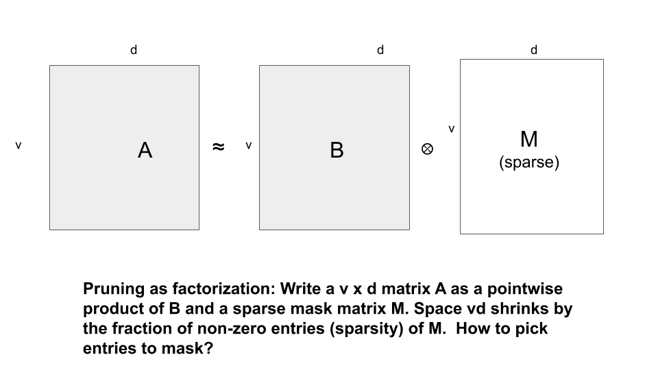
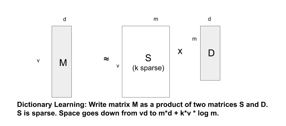
Low Rank Approximation: Another common approach is error |A-UV^T|_F where U, V are low rank (say rank k) matrices. This minimization can be solved optimally by using ; this is useful for embedding tables that are tall and thin and thus already have a low rank to begin with -- dictionary learning exploits the possibility that even though the number of embedding entries may be large there may be a smaller dictionary of basis vectors such that each embedding vector is some sparse combination of a few of these dictionary vectors -- thus it decomposes the embedding matrix into a product of smaller dictionary table and a sparse matrix that specifies which dictionary entries are combined for each embedding entry.

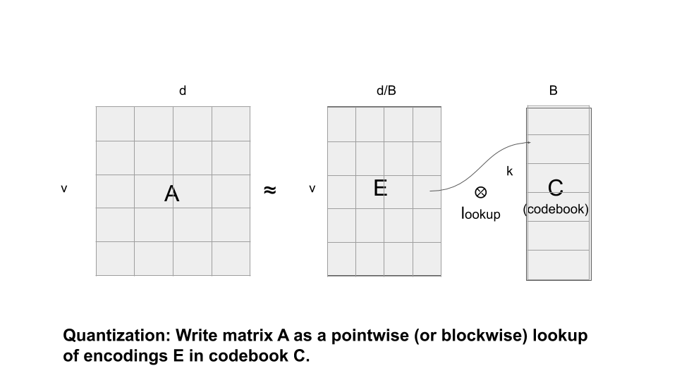
The commonly used where each entry or a block of entries is quantized by possibly rounding the entries into a small number of bits so that each entry (or a block of entries) gets replaced by a quantized code. Thus the original matrix gets decomposed into a codebook and an encoded representation; each entry in the original matrix is obtained by looking up the code in the encoding matrix in the codebook. Thus it can again be viewed as a special product of the codebook and the encoding matrix. The codebook can be computed by some clustering algorithm (such as k-means) on the entries or blocks of entries of the matrix. This is in fact a special case of dictionary learning with sparsity one as each block is being expressed as one of the vectors in the codebook (which can be viewed as the dictionary) instead of a sparse combination. Pruning can also be viewed as a special case of quantization where each entry or block is pointing to a codebook entry that is either zero or itself.

Thus there is a continuum from pruning to quantization to dictionary learning and they are all forms of matrix factorization just as low-rank-approximation.

Factorization as Mutation

Applying these different types of matrix factorizations can be viewed as mutating the network architecture by splicing a layer into a product of two layers.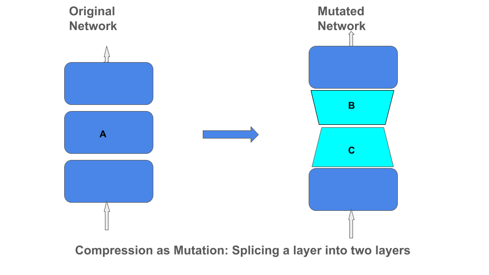

Tensorflow Matrix Compression operator

Given the wide variety of matrix compression algorithms it would be convenient to have a simple operator that can be applied on a tensorflow matrix to compress the matrix using any of these algorithms during training. This saves the overhead of first training the full matrix, applying a factorization algorithm to create the factors and then creating another model to possibly retrain one of the factors. For example, for pruning once the mask matrix M has been identified one may still want to continue training the unmasked entries. Similarly in dictionary learning one may continue training the dictionary matrix.

We have that is faster than the method that not only takes into account the magnitude of the entries to decide which ones to prune but also its effect on the final loss by measuring the gradient of the loss with respect to the entry.

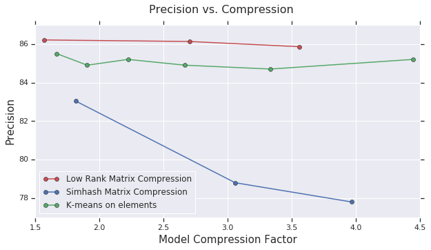
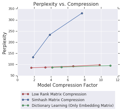
Thus we are performing a mutation of the network in real time where in the beginning there is only one matrix and in the end this produces two matrices in the layer. Our factorization methods need not even be gradient based but may involve more discrete style algorithms such as hashing, -- the matrix to be compressed is multiplied by a random projection matrix and the entries are rounded to binary values -- thus it is a factorization into one random projection matrix and a binary matrix. The following plots show how these algorithms perform on compressing models for . The results show that while low-rank-approximation beats simhash and k-means on CIFAR10, on PTB dictionary learning is slightly better than low-rank-approximation.

CIFAR10

PTB

Conclusion

We developed an operator that can take any matrix compression function given as a factorization and create a tensorflow API to apply that compression dynamically during training on any tensorflow variable. We demonstrated its use via a few different factorization algorithms including dictionary learning and showed experimental results on models for CIFAR10 and PTB. This also demonstrates how we one can dynamically combine discrete procedures (such as sparse matrix factorization and k-means clustering) with continuous processes such as gradient descent.

Acknowledgements

This work was made possible by the contributions of several people including Xin Wang, Badih Ghazi, Khoa Trinh, Yang Yang, Sudeshna Roy and Lucine Oganesian. Also thanks to Zoya Svitkina and Suyog Gupta for their help.