Posted by Emily Fertig, Joshua V. Dillon, Wynn Vonnegut, Dave Moore, and the TensorFlow Probability team
In this post, we introduce new tools for variational inference with joint distributions in for parameters of a regression model to estimate the effects of various treatments or observed features on an outcome of interest. Credible intervals bound the values of an unobserved parameter with a certain probability, according to the posterior distribution of the parameter conditioned on observed data and given an assumption on the parameter's prior distribution.
In this post, we demonstrate how to use VI to obtain credible intervals for parameters of a Bayesian linear regression model for radon levels measured in homes (using in Stan). We demonstrate how TFP JointDistributions combine with bijectors to build and fit two types of expressive surrogate posteriors:
a standard Normal distribution transformed by a block matrix. The matrix may reflect independence among some components of the posterior and dependence among others, relaxing the assumption of a mean-field or full-covariance posterior.
a more complex, higher-capacity
You can follow along and see all the details in this . We are interested in credible intervals for the effect of location (county) on the radon level of houses in Minnesota. In order to isolate this effect, the effects of floor and uranium level are also included in the model. Additionally, we will incorporate a contextual effect corresponding to the mean floor on which the measurement was taken, by county, so that if there is variation among counties of the floor on which the measurements were taken, this is not attributed to the county effect.
The regression model is specified as follows:
and .
Variables are defined for the deterministic parameters and the Normal distribution scale parameters, with the latter constrained to be positive.
PYTHON
import tensorflow as tf import tensorflow_probability as tfp tfd = tfp.distributions tfb = tfp.bijectors
Suppose we have the following generative process, where ? represents random parameters (uranium_weight, county_floor_weight, and county_effect in the regression model) and ω represents deterministic parameters (floor_weight, log_radon_scale, county_effect_scale, and bias). The x? are features (log_uranium, floor_of_house, and floor_by_county) and the ?? are target values (log_radon) for ? = 1...n observed data points:
(Technically we're assuming q is .)
Since the bound holds for all q, it is obviously tightest for:
for more information on variational inference.
Expressive surrogate posteriors
Next we estimate the posterior distributions of the parameters using VI with two different types of surrogate posteriors:
A constrained multivariate Normal distribution, with covariance structure induced by a blockwise matrix transformation.
A multivariate standard Normal distribution transformed by an for the parameters.
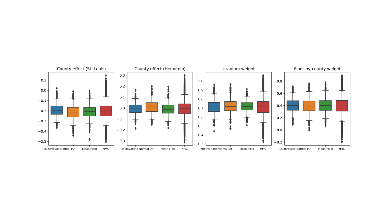
The box-and-whiskers plots below show 50% and 95% credible intervals for the county effect of the two largest counties and the regression weights on soil uranium measurements and mean floor by county. The posterior credible intervals for county effects indicate that location in St. Louis county is associated with lower radon levels, after accounting for other variables, and that the effect of location in Hennepin county is near neutral.
Posterior credible intervals on the regression weights show that higher levels of soil uranium are associated with higher radon levels, and counties where measurements were taken on higher floors (likely because the house didn't have a basement) tend to have higher levels of radon, which could relate to soil properties and their effect on the type of structures built.
The (deterministic) coefficient of floor is -0.7, indicating that lower floors have higher radon levels, as expected.
Mean-field surrogate posterior
VI surrogate posteriors are often assumed to be mean-field (independent) Normal distributions, with trainable means and variances, that are constrained to the support of the prior with a bijective transformation. We define a mean-field surrogate posterior in addition to the two more expressive surrogate posteriors, using the same general formula as the multivariate Normal surrogate posterior. Instead of a blockwise lower triangular linear operator, we use a blockwise diagonal linear operator, in which each block is diagonal:
In this case, the mean field surrogate posterior gives similar results to the more expressive surrogate posteriors, indicating that this simpler model may be adequate for the inference task. As a “ground truth”, we also take samples with Hamiltonian Monte Carlo (see the
Conclusion
In this post, we built VI surrogate posteriors using joint distributions and multipart bijectors, and fit them to estimate credible intervals for weights in a regression model on the radon dataset. For this simple model, more expressive surrogate posteriors appeared to perform similarly to a mean-field surrogate posterior. The tools we demonstrated, however, can be used to build a wide range of flexible surrogate posteriors suitable for more complex models.
Check out our code, documentation, and further examples on the TFP home page.
Vollständiger Original-Bericht
Ausführliche Details, Code-Beispiele & Hersteller-Stellungnahme auf blog.tensorflow.org.

SOCIAL SHARE CARD GENERATOR