A guest post by James Bartlett and Zain Asgar of Pixie.
, our goal is to enable developers to quickly understand and debug production systems. We achieve this by providing developers easy access to an assortment of metric and log data from their production system. For example, we collect structured information about CPU and memory usage for each process in their system, as well as many types of unstructured data (for example, the body of an HTTP request, or the error message from a program).
These are just two examples, we collect many other types of data, as well. For this blog post, we will focus on the vast amounts of unstructured data we collect in Pixie such as HTTP request/response bodies. We foresee a future where this unstructured machine data can be queried as easily and efficiently as the structured data. To achieve this, we leverage state-of-the-art NLP techniques to learn the structure of the data.
In this article, we’d like to share our experience and efforts here, in the hopes they are useful to inform your thinking on similar problems.
HTTP clustering
Suppose a developer using Pixie wanted to get an idea of which types of HTTP requests are particularly slow. Instead of forcing the developer to sift through many individual HTTP requests by hand, we can instead cluster the HTTP requests semantically and then show them a timeseries of latencies for each type of semantically clustered request. To demonstrate this, let’s walk through the end result and then we’ll come back to how we got to this point. We will use Pixie to explore a demo application called
As you can see in the service graph, there’s a frontend service that handles incoming requests and sends them to their respective microservices. So let’s delve into the HTTP requests sent to the frontend service and their corresponding latencies.
From this small sample of requests, it's not immediately clear what’s going on. It looks like the requests with `email=...?address=...` are much slower than the others, but we can’t be sure these examples weren’t just outliers. Instead of looking at more data, let’s use our soon-to-be-explained unstructured text clustering techniques, to cluster the HTTP requests semantically by the contents of their bodies.
dataset to bootstrap our model training. This dataset is a collection of log messages from various contexts (Android sys logs, Apache Server logs, supercomputer/HPC logs, etc). To test the models generalization to unseen log formats, we reserved the Android log data for testing, and trained on the remainder of the log data.
We use Google’s
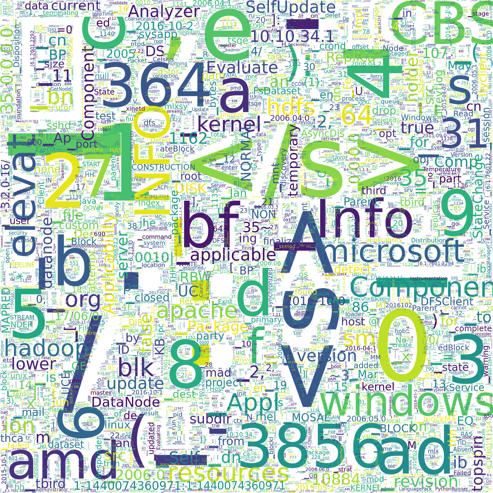
Word cloud showing vocabulary subword pieces from Logpai Loghub machine log dataset tokenization.
This word cloud provides insight into the biases of our dataset. For example, about 30% of the data is Windows logs, as you can see by the high frequency of the token “windows”, and “microsoft”. Also, if you have a keen eye, you might think we have a lot of frowny faces in our data set, but in fact “):” is almost always preceded by an opening parenthesis, as in the following examples:
PYTHON
[Thu Jan 26 12:23:07 2006] [error] config.update(): Can't create vm
[Fri Jan 27 11:55:16 2006] [error] [client 202.143.128.18] client sent HTTP/1.1 request without hostname (see RFC2616 section 14.23): /
Model Architecture
Using this tokenized dataset, we train a self-attention based model using left-to-right next word prediction (à la OpenAI's GPT models). Left-to-right next word prediction is the task of trying to predict the next token given a sequence of prior context tokens. The left-to-right part distinguishes it from BERT style models that use bidirectional context (we will try bidirectional models in the future). This
GPT-style language model architecture
All in all, this architecture has 6.47M parameters, making it quite small in comparison to state-of-the-art language models. DistillBERT, for instance, has 66M parameters. On the other hand, the largest version of GPT-3 has 175B parameters.
We trained this architecture for 10 epochs with roughly 100 million unique log messages per epoch. After each epoch, we ran the model on a validation set and the model from the epoch with the highest validation accuracy was used as the final model. We achieved a test accuracy of 63.13% for next word prediction on the holdout Android log data. Given that we haven’t yet explored hyperparameter tuning, or other optimizations, this level of accuracy is a promising starting point.
We now have a way to predict future tokens in machine log data from context, with somewhat decent accuracy. However, this doesn’t immediately help us with our original goal of extracting structured features from the data. To further this goal, we will explore the feature space generated by the language model, rather than the predictions of the language model.
The goal is to transform our complicated data space into a fixed-dimensional feature space which we can then use for subsequent tasks. In order to do this we need to transform the outputs of the language model into a fixed-dimensional vector, which we will call the feature vector. One way to do this comes from
Alammar, J (2018). The Illustrated Transformer [Blog post]. Retrieved from data that I’ve hand labeled into semantic clusters. Below are three of the log messages in the hand labelled test data set. The first two are labelled to be in the same semantic cluster, since both relate to failures to find files, the last is from a different cluster, since it's an unrelated message about flushing data.
PYTHON
[Wed Nov 09 22:30:05 2005] [error] [client 216.138.114.25] script not found or unable to stat: /var/www/cgi-bin/awstats.p

[Sat Jan 28 19:29:29 2006] [error] [client 211.154.174.50] File does not exist: /var/www/html/modules

20171230-12:25:37:318|Step_StandStepCounter|30002312|flush sensor data
Using the hand-labelled test set, we can measure how well the model separates the different clusters. To do this, we use the KMeans algorithm to generate a clustering based on the output of the model, and then compare this clustering to the hand-labelled clustering. On this test set, the model’s adjusted rand score, a metric where 0.0 is random labelling and 1.0 is perfect labelling, was 0.53. As with next word prediction accuracy, the performance isn’t great but a good starting point.
We can also view a low-dimensional representation of the feature space for the model, using PCA to reduce the dimensionality to two. The figures below show the first two PCA dimensions of the embeddings for each point in the test data set. The colors represent the semantic cluster the point belongs to. Note that since these are plots in a two-dimensional subspace of the embedding space, the absolute position of points carries little meaning, more meaning is derived from the tightness of each of the clusters. In the figure below, we can see that the model separates some of the classes reasonably well, but fails on others.
(a script in Pixie’s scripting language based on Python/Pandas) to cluster our data. We are working on a public API to load in custom ML models into the engine, but for now we will use some internal features to do that. Once the model is loaded in, we can use it on any unstructured data in the Pixie Platform.
Some of the areas we are currently exploring include our vision of federated differentially-private training of models, bidirectional language models ala BERT, compression schemes for unstructured data based on learned structural representations of the data, and anomaly detection on unstructured data
Our goal on the Pixie ML team is to harness ML to simplify developers' access to monitoring data, while operating in heterogeneous edge environments. If any of this interests you, or you have other questions feel free to join our is an open-source project that gives you instant visibility into your application. It provides access to metrics, events, traces and logs without changing code. Pixie is in the process of being contributed to the is the GM/GVP of Pixie and Open Source at New Relic. He is also an Adjunct Professor of Computer Science at Stanford University. He was the Co-founder/CEO of Pixie Labs.
Vollständiger Original-Bericht
Ausführliche Details, Code-Beispiele & Hersteller-Stellungnahme auf blog.tensorflow.org.

SOCIAL SHARE CARD GENERATOR