📚 How to Set Started with TensorFlow Using Keras API and Google Colab

Step-by-step tutorial to analyze human activity with neuronal networks

This beginner tutorial aims to give a brief overview of the fundamentals of TensorFlow and to guide you through a hands-on project. The tutorial might be of value to you, if:

• you have built your first traditional machine learning models and now you are curious about how to get started with your first TensorFlow model.
• you have explored the basic concepts of TensorFlow already but you are looking for a practical challenge to improve your skills.

In case you are completely new to data science or machine learning models, I recommend focusing on other tutorials first as it will be crucial to have a basic understanding first.

This article is structured into three main sections:

#1 Brief introduction to TensorFlow and Keras API
#2 Tutorial on how to set up TensorFlow using Google Colab (for free)
#3 Hands-on project: Human activity classification

#1 Brief introduction to TensorFlow and Keras API

If you are completely new to TensorFlow, I recommend the following video, where the main concepts and different layer structures are explained in a short but good way. This is not a comprehensive lecture, but it gives a good introduction to the topic itself.

While TensorFlow is the underlying Machine Learning platform, Keras on the other side is an API that will help you to set up your models in a fast way and reduces the manual coding effort.

Keras is a deep learning API written in Python, running on top of the machine learning platform TensorFlow. It was developed with a focus on enabling fast experimentation. Being able to go from idea to result as fast as possible is key to doing good research. [https://keras.io/about]

The development team states that Keras is:

• Simple — but not simplistic. Keras reduces developer cognitive load to free you to focus on the parts of the problem that matter.
• Flexible — Keras adopts the principle of progressive disclosure of complexity: simple workflows should be quick and easy, while arbitrarily advanced workflows should be possible via a clear path that builds upon what you’ve already learned.
• Powerful — Keras provides industry-strength performance and scalability: it is used by organizations and companies including NASA, YouTube, and Waymo.

[again sourced from https://keras.io/about]

#2 Tutorial on how to set up TensorFlow using Google Colab (for free)

A good piece of advice to use TensorFlow is to run it on a Graphics Processing Unit (GPU) or Tensor Processing Unit (TPU) instead of a normal Central Processing Unit (CPU) accelerator. While simple models and calculations might still work using a CPU, you might notice that the full capability of TensorFlow can only be appreciated on graphical hardware.

The easiest and most straightforward way to make use of a GPU is the usage of Google Colaboratory (“Colab”) which is somewhat like “a free Jupyter notebook environment that requires no setup and runs entirely in the cloud.” While this tutorial claims more about the simplicity and advantages of Colab, there are drawbacks as limited GPU hours and reduced computing power compared to proper cloud environments. However, I believe Colab might not be a bad service to make the first steps with TensorFlow.

To set up a basic environment for TensorFlow within Colab you can follow the next few steps:

1. Open https://colab.research.google.com/ and register for a free account
2. Create a new notebook within Colab
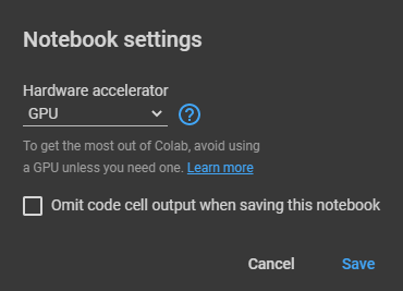
3. Select Runtime from the menu and Change the runtime type
4. Choose GPU from the Hardware accelerator options - click save

Now you can import TensorFlow and check that everything is set with the following few lines of code:

You should see as output now a version displayed (e.g. “2.5.0”) as well as a physical device message that indicates GPU usage. Your Notebook is now ready to use TensorFlow in practice!

#3 Hands-on project: Human activity classification

The following tutorial aims to analyze a dataset on human activity classification. The dataset consists of time series recordings from the inertial sensors of smartphones that are carried by people performing different activities.

Background & dataset information

It is interesting to understand if simple smartphone measurements could be used to classify the physical activity a human is doing. The six activity classes are the following:

1. Walking
2. Walking upstairs
3. Walking downstairs
4. Sitting
5. Standing
6. Laying

A short video describing the measurement and the different activities can be found here:

The outcome of such sensor-based classification models could be used by health applications or other smartphone apps to improve the user experience, to suggest activities based on the current recordings, or to track physical activities during the day.

The given dataset consists of measurements from the inertial sensors of smartphones that are carried by people performing different activities. In total, the dataset contains 10,299 entries and is split into 70% training data (7,352 entries) and 30% test data (2,947 entries). The sensor signals (accelerometer and gyroscope) were pre-processed by applying noise filters and then sampled in fixed-width sliding windows. Each signal was recorded for the three coordinates (x, y, z) and can be seen as time series recording having 128 timestamps with their corresponding value. The target column contains the activity labels: WALKING, WALKING_UPSTAIRS, WALKING_DOWNSTAIRS, SITTING, STANDING, LAYING.

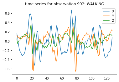
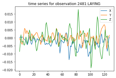
All features of the training and test dataset are numeric (float), normalized, and bounded within -1 and 1. Two example measurements along the 128 timestamps are present in Figure 1. It is shown that each human activity has its characteristics across the three coordinates and over time. Hence, there is a chance to identify patterns and trends within the time series that indicates the activity class.

More information about the dataset and the background can be found in the readme file or on this website.

Step 01: Initial load of data & required libraries

To get started with the project, it is required to load the dataset into the Colab environment. Don’t worry too much about the code below, it just moves all the required files into your workspace:

Not surprisingly, we need to import some required libraries to make our life easier. A vital library here is of course TensorFlow itself:

To simplify our tutorial, we will use only the available body data from the inertial signals. The dataset is already split into training (7352 entries) and test (2947 entries) datasets along 128-time series measurements and across 3 coordinates. To get proper datasets in the format of (n, 128,3), we can use the following code:

One last important step for preparation is the transformation of our target variables into a one-hot-encoded measurement. Instead of having a numerical value that indicates the categories (e.g. 0 = WALKING), we end up with having arrays, that contain the probability for each of the available categories (e.g. [1, 0, 0, 0, 0, 0] = WALKING or [0, 0, 0, 1, 0, 0] = SITTING) where there is a 100% probability for the corresponding category in this case. This is important as TensorFlow will calculate the probability for each of the possible categories for us. Hence, we need to prepare the training data accordingly. The Keras API has a simple built-in function designed for that requirement. You will notice, that the shape of the target variable has changed from (n,) to (n, 6):

Step 02: Plot some example time series

In this tutorial, we will ignore a proper exploratory analysis section as we want to focus more on the usage of TensorFlow. However, it might make sense to plot some example time series at this stage, as it will give us a better understanding of the data that we would like to analyze for classification.

We can now use the following code to plot some random measurements from the dataset. I have selected measurements 992 (walking) and 2481 (laying) to demonstrate the differences in the data:

The output can be seen below. You might identify already some differences in the human body measurements, depending on the underlying activity. Finally, it is our hope and chance to run a neuronal network model on the data that might predict our activity classes well. Let’s see!

Step 03: Build and train a neuronal network using Keras API

To build and train neuronal networks in TensorFlow you need to split your available training data into training and validation subsets. TensorFlow will then use both to train the model and assess the progress using the validation loss and validation accuracy. You can vary the size of the accuracy data set but I used 20% of the original training data in this case. The random state can be set to reproduce recognizable data splits at different times.

A best practice to monitor your model development through the training process is to set up TensorBoard. You can prepare your notebook with the following code, where you load the extension and create a log writer:

To set up the neuronal network, you first need to decide what type of network you want to build. The simplest architecture is a linear stack of layers called a sequential model. You can create a sequential model by passing a list of layer instances to the constructor. To get started, you initiate your model:

model = tf.keras.Sequential()

From this point, it is up to you to add any layers you would like to use. There exist good tutorials on the web that describe the different functionality of the layers. For this tutorial, we will only guide you through a simple working setup to let you run your first model successfully. Feel free to add and modify the architecture to beat my accuracy!

Firstly, we add the input layer having the dimensions of our data set (128,3):

model.add(tf.keras.layers.InputLayer(input_shape=(128,3)))

Secondly, we add a one-dimensional convolutional layer where we can set parameters for the number of filters and the kernel size. This layer will be followed by a Batch Normalization layer that will transform inputs so that they are standardized, meaning that they will have a mean of zero and a standard deviation of one

model.add(tf.keras.layers.Conv1D(filters=256, kernel_size=10))

model.add(tf.keras.layers.BatchNormalization())

Thirdly, we add a ReLu layer and a Global Average Pooling layer. Finally, we need a Dense layer that activates our network into a six-class category output. Since we have a classification problem, we use the softmax activation function with six units (as we have six categories).

model.add(tf.keras.layers.ReLU())

model.add(tf.keras.layers.GlobalAveragePooling1D())

model.add(tf.keras.layers.Dense(units=6, activation=tf.nn.softmax))

To train the model, we need to compile the model first with an appropriate optimizer. For our tutorial, I have selected the Adam optimizer where you can vary the learning rate.

model.compile(optimizer=tf.keras.optimizers.Adam(0.001), loss='categorical_crossentropy', metrics=['accuracy'])

To fit the model, we need to decide on how many epochs and on what batch size we want to run it. An epoch is the time step that is incremented every time it has gone through all the samples in the training set. The batch size is the number of data entries for every batch. To link our model to the TensorBoard monitoring, we add a callback and set the log directory.

callbacks = [tf.keras.callbacks.TensorBoard(log_dir=logdir)]

model.fit(x_train, y_train, epochs=100, batch_size=32, callbacks=callbacks, validation_data=(x_valid, y_valid))

When you run the code, you will see some output below your cell that gives you an indication of every training epoch. In TensorBoard you will be able to see the increasing accuracy as well as the decreasing loss for both, the training and the validation data. Once the training has run through all epochs it will stop automatically. The whole code for the model fitting is stated below:

Let us now try to understand what we have built and how the model developed over time during the training process. As you can see in the below screenshots, there is a significant improvement along the first 20 to 30 epochs and a moderate improvement afterward. The blue line indicates the accuracy and the loss for the training data set. The red line represents the validation data.

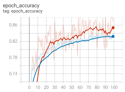
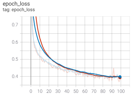
Overall, we did not do too badly and achieved a validation accuracy of 85.38%. A comparable development between training and validation loss indicates a non-overfitted training procedure. However, there is a chance to improve our model further. Feel free to explore this on your own. Some ideas are the following:

• play with the number of epochs, the batch size, and the learning rate
• modify the amount of filter and kernel size in the Conv1D layer
• add more layers and play around with different architectures
• add the other data set to the model (besides the body data only)

Finally, it is always the last step to assess the accuracy of the model on the test data set. So far, we trained the model using only the training and validation data. To apply our final model to the test data set you can use the code below. We calculate the probabilities for each of the six classes using our model. Afterward, we take the maximum probability per row and identify therefore the discrete class for that row.

The test accuracy in my approach showed 84.42% and is therefore a bit lower than the validation accuracy, but on a similar level to the training accuracy.

Congratulations: you applied your first neuronal network using TensorFlow!

Please note that you will achieve different accuracy and loss values as TensorFlow cannot be reproduced in the same way. However, I expect your values to be around a range between 75% and 90%.

Summary

The idea of the above tutorial was to give you a practical hands-on idea to get started with TensorFlow and the Keras API. I am aware that it is not even close to a proper explanation or detailed description of the features. However, I hope this might help some beginners to run their first model on their own and to understand the basic pieces of the puzzle around TensorFlow.

Of course, there is so much more to explore. Try to beat our initial accuracy achievements and drop a comment with your achievement!

References

Reyes-Ortiz,Jorge, Anguita,Davide, Ghio,Alessandro, Oneto,Luca & Parra,Xavier. (2012). Human Activity Recognition Using Smartphones. UCI Machine Learning Repository

This used dataset is licensed under a Creative Commons Attribution 4.0 International (CC BY 4.0) license. This allows for the sharing and adaptation of the datasets for any purpose, provided that the appropriate credit is given.

For further information please visit this site.

How to Set Started with TensorFlow Using Keras API and Google Colab was originally published in Towards Data Science on Medium, where people are continuing the conversation by highlighting and responding to this story.