

 800+ IT
News
als RSS Feed abonnieren
800+ IT
News
als RSS Feed abonnieren📚 Kernels: Everything You Need To Know
💡 Newskategorie: AI Nachrichten
🔗 Quelle: towardsdatascience.com
👨🏫 Mathematics
Kernels: Everything You Need to Know
Density Estimation, Dot Products, Convolutions and everything…
Kernels or kernel functions are beautiful mathematical concepts that are used in machine learning and statistics with different forms. If you’re a beginner you might feel tempted to know the exact definition of kernels, but you may get confused by multiple definitions of kernels that are explained across blogs/websites on the internet.
The kernel function is a confusing concept, just because the knowledge around it is decentralized across its applications and a common intuition connecting them is missing. This (huge) blog undertakes the motive of unifying all knowledge on kernels used in different ML applications. Just as most beginners, the kernel function kept me in a state of confusion for a long time, until I developed an intuition that would connect all links.
We begin our journey with non-parametric models, then we start discussing different types of kernels and their typical applications across statistics and ML. Similar to kernel functions, I have an attempt to explain PCA mathematically, considering all perspectives. You may have a read:
Principal Component Analysis: Everything You Need To Know
https://medium.com/media/2ddb5bb30a41babc4869c8930f80c011/hrefNon-Parametric Models
Non-parametric models are those statistical models that do not have parameters which grow with the size of the input. Note, non-parametric models do not mean ‘model with zero parameters’ but they work with a fixed set of parameters, also called hyperparameters, which do not increase with the increase in the dimensionality of the inputs. A vanilla linear regression model, has parameters θ that determine the slope of the hyperplane whose size depends on the dimensionality of the input x,
https://medium.com/media/db59710fd3073101d6beb74ac0c221b0/hrefNext, consider the KNN model, where we determine the class of a test sample by analyzing the classes of its K nearest neighbors. If K = 1, we assume that the test sample belongs to the same class as that of the nearest neighbor. This model does not have any parameters that would grow with the dimensionality of the inputs. For a vanilla implementation, we would only need a single parameter, K, even if we working with large inputs (in terms of dimensionality).
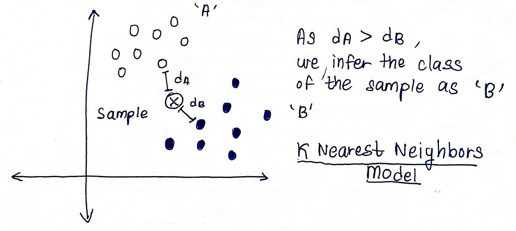
KNN is a non-parametric model which has a hyperparameter K, provided by the user. Non-parametric might seem to an obvious-choice at the first glance, as,
They make no prior assumptions regarding the distribution of the data. For instance, in case of vanilla linear regression, which is a parametric model, we assume that the conditional distribution of Y (dependent variables) given X (features) is a Gaussian Distribution whose mean is a linear combination of the features (where weights are θ) and variance equal to σ²https://medium.com/media/f14bf24212a0d8da71ef6bc84ce19193/href
which might not hold always, because,
For each test sample, they need to keep the entire training data in memory, which is also true for the KNN model. For each sample, we need to calculate its distance from each training sample, so we need to retrieve/store each sample in memory, which might not be feasible to large datasets or even smaller datasets which a large number of features.
The basic idea around non-parametric models is to gather some useful insight from the data and use to solve the given problem, without encoding information about the data in tunable parameters.
Next, we move on to kernels, that have different use-cases across ML, and differ slightly with their meanings in each context. So far, after researching for this blog, and also from my previous attempts of understanding kernels as a whole, I feel that kernels are machines that provide information on the neighbors of a given datapoint (as an input to the machine). This local information i.e. the information on datapoints that lie in the proximity of the datapoint under consideration, is then used to the given problem. Once we use the kernel function on each of the datapoints, we can get a clear picture of what’s going on in the locality of the data.
We’ll explore these three aspects of a kernel, which are three different concepts with their major applications in ML,
Density Kernels: Use of Kernels for Density Estimation
Density kernels, kernel density estimation, kernel regression
We can use kernels to estimate the probability density for a given test sample, by modelling the underlying probability distribution with the training samples. The terms ‘test’ sample and ‘training’ samples simply refer to unobserved and observed samples respectively, considering ML lingo.
For continuous random variable X, we can integrate the probability density function of X within a suitable range, say, from x_1 to x_2, and we get the probability of X assuming a value in the range [ x_1 , x_2 ]. If you aren’t comfortable with the topic of probability density or random variables, here’s my 3-part series on probability distributions,
https://medium.com/media/a77035a3d37ac962cbf5660473dc2262/hrefDensity Kernels and Kernel Density Estimation (KDE)
Let us start our discussion with a problem. Dr. Panchal lives in a crowded city block which is surrounded by houses on all sides. The local police have hired a detective whose job is to determine the number of persons who reside in the doctor’s house or who are his family members, just to make sure things are going well. The detective could not ring the doctor’s bell and ask how many family members reside there, as it would warn the doctor if there’s something suspicious.
The detective would start by interrogating the houses that are adjacent to Dr. Panchal’s house, as they could have a clear sight of what’s in there. The detective is expected to give a higher weight/importance to the information gained from these direct neighbors. Next, in order to gain more insights, the detective interrogates houses that are slightly farther away that do not have a direct sight of Dr. Panchal’s house but might have good information of their neighbor. The detective would give lesser importance to the information received from these neighbors, as their observations might not be that correct as that of the direct neighbors (whose houses are adjacent to Panchal’s). The detective performs several such rounds reducing the importance, moving away from Dr. Panchal’s house.
A density kernel does something similar to capture neighboring information around a given point. If we’re given a dataset D with N samples where each sample is a real number,
https://medium.com/media/72ee2f55eca936f29e498113b01cd2bd/hrefThe kernel in the above snippet is an Epanechnikov (parabolic) kernel. The kernel function has some special properties here,
https://medium.com/media/3904dd62b537f3da1d63403439917184/href- Property 1: The kernel function or the detective does not matter in which direction the x or some neighbor’s house lies. Information gained from two houses to the right or two houses to the left is the same.
- Property 2: The kernel function represents a valid PDF and it integrates to 1 over the entire real domain.
- Property 3: Support of a kernel is the set of all values u such that K( u ) is not equal to 0. It represents the coverage area of the detective from where some non-zero importance will be given to information gathered. If the detective decides to interrogate in all houses in a radius of 5 km, the support would be all houses within that 5 km circle.
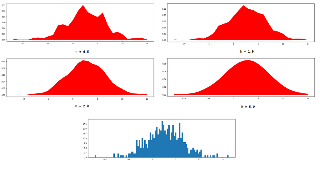
Every type of kernel will perform a similar task of encoding neighboring information, which each one will have a different strategy to do so. Unlike our detective, who slowly reduced the importance of interrogation as he moved away from Dr. Panchal’s house (a Gaussian kernel would do that), another detective might just continue giving equal importance to all interrogations, neglecting the distance upto a certain extent (a uniform kernel). Imagine, that from our dataset D, the distribution of all x_i is,
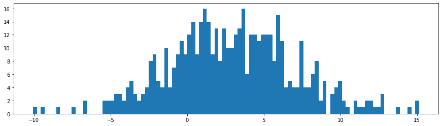
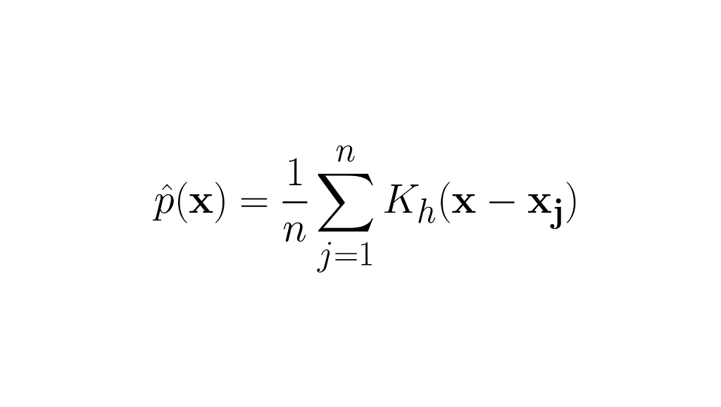
Our goal is to create an estimate of the probability distribution of X. We’ll do this by estimating the density at each sample x_i and using the kernel to collect neighboring information,
https://medium.com/media/152a3a34de15b564f525abd6d8cbd8da/href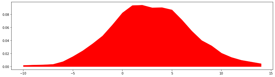
If x_i is away from x, | x — x_i | will have a larger value thus yielding a very small value for K( x — x_i ) and reducing the say of x_i in the determination of probability density at x. The parameter h is the smoothing parameter called the bandwidth of the kernel. Greater the value of h, smoother will be predicted probability density.
Kernel Regression
Kernel regression is a non-parametric version of the linear regression model where we model the conditional expectation of the outcome variable. In the case of simple linear regression, we model the conditional expectation E[ Y | X ] directly by expressing it as a linear combination of the independent variables. This gives rise to a discriminative model, whereas kernel regression is a generative model, as we’re modelling the joint probability distribution P( X , Y ) and P( X ) by the means of kernel density estimation.
https://medium.com/media/254b7cd80cf7e159feb1b37e94190420/hrefOn observing the resultant expression, you’ll realize that the predicted outcome y_hat is a weighed combination of all y_i, where the weights are determined by the values of the kernel function for all x_i.
Mercer Kernels: Dot Products in Higher Dimensions
Mercer kernels and positive definiteness, use of Mercer kernels in SVM
Mercer Kernels or Positive definite kernels are functions that take in two inputs and produce a real number which characterizes the proximity of the two inputs (or their high-dimensional representations) in some other space. It turns out that these kernels are useful from the computational perspective as they help us compute dot products of vectors in a high-dimensional without explicitly performing any transformation to bring our own vectors into that high-dimensional space.
Mercer Kernels
Let us start our discussion by defining the kernel function and some of its properties,
https://medium.com/media/fe97258d7958e650d791ed755afdf296/href- The Mercer kernel is a function that takes in two datapoints from our dataset D, and outputs a real number that represents the proximity of these two datapoints in the feature space.
- If we have n datapoints in our dataset D, and we run our Mercer kernel on each pair of datapoints and arrange the resulting outputs in a matrix, we achieve a positive definite matrix. This matrix, that depicts the similarity amongst the datapoints, is called the Gram Matrix.

Positive definite matrices are special, considering their spectral properties. They have positive eigenvalues and the corresponding eigenvectors form an orthonormal basis. We have a special property, for mercer kernels, using which the value of the kernel function as be expressed as the dot product of two transformed vectors,

One might have an urge to feel the intuition behind this statement, but it lives in the sanctum of Hilbert Spaces which deserves a separate blog. For time being, its good to understand that the value of the kernel function, with two input vectors, as be described as the dot product of some other two vectors that lie in higher dimensional.
Mercer kernels provide a shortcut for computing the dot product between those two high-dimensional vectors without explicitly computing those vectors. Hence, we can leverage the advantages of high-dimensional spaces are sometimes useful in machine learning, especially when samples are not linearly separable.
For some optimization problems, like the one encountered while optimizing SVMs, we’ll need to compute dot products between two transformed samples which are two high-dimensional vectors. The use of kernel functions will help us compute this dot product easily without performing any explicit transformations on the samples.
Use of Mercer Kernels in SVMs
SVMs are linear classifiers that fit a hyperplane such that a decision boundary is formed between samples of two classes. To determine the best hyperplane i.e. the hyperplane which divides the samples into two classes and maximizes the ‘margin’, we need to solve an optimization problem that contains an objective function (a function which is either maximized or minimized) given some constraints on the parameters of the objective.
The derivation of the SVM optimization problem is covered in these blogs extensively by Saptashwa Bhattacharyya so reading them once would help us proceed further,
Understanding Support Vector Machine: Part 2: Kernel Trick; Mercer’s Theorem
The vectors w and b characterize the hyperplane which forms the decision boundary. The margin/width between the support vectors is given in the first expression below. Also, we would match the predictions made by the SVM and the target labels, or more precisely, the sign of w.xi + b and yi,

The optimization problem that we have to solve for an optimal decision boundary is,

We solve this optimization problem with Lagrangian multipliers, so the first step would be build a Lagrangian and equating the partial derivatives w.r.t. its parameters to zero. This would yield an expression for w which minimizes the Lagrangian.

After substituting these results into the Lagrangian, we obtain an expression which clearly depicts the role of kernel functions,

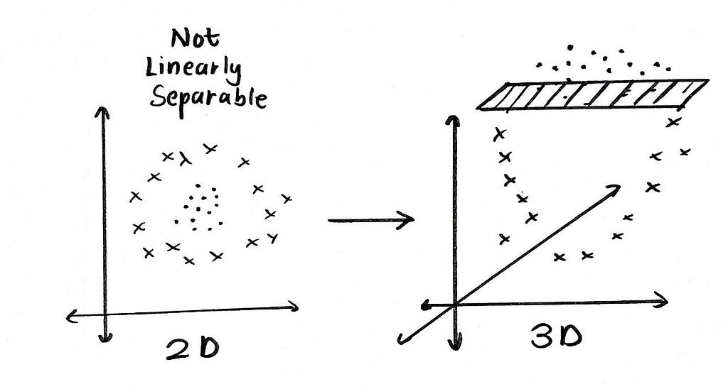
In order to achieve the optimal hyperplane, we need to compute the dot product between pairs of samples from our dataset. In some cases, finding an optimal hyperplane isn’t possible, as the samples may not be linearly separable i.e. the samples couldn’t be divided into two classes by merely drawing a line/plane. We can increase the dimensionality of the samples, by which we can discover a separating hyperplane easily.
<img>
Consider a feature map ϕ, that transform the data sample x into a higher dimensional feature i.e. ϕ( x ). In the Lagrangian of the SVM, if we use these features instead of the data samples, we need to compute,

We can replace the dot product of the features with a kernel function that takes into two data samples (not transformed features),

This technique is popularly known as the kernel trick and is a direct consequence of Mercer’s theorem. We’re able to calculate the dot product of two high-dimensional features without explicitly transforming the data samples to that high-dimensional space. With more dimensions, we have greater degrees of freedom for determining the optimal hyperplane. By choosing different kernels, the dimensionality of the space in which are features lie, can be controlled.
The kernel function has a simpler expression to be evaluated, like the ones listed below,

Kernels For Convolutions: Image Processing
Kernels used in convolutions and image processing
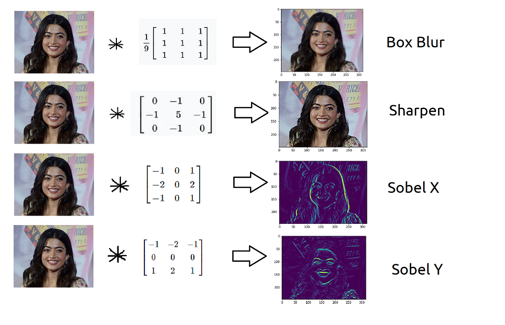
Kernels are fixed-size matrices that are convolved across an image or a feature map to extract useful information out of it. In image processing lingo, a kernel matrix is also called a convolution matrix, and it used to perform operations on an image. Each kernel has a specialized operation of its own, which transforms the image after the convolution.
Convolutions and Kernels
Convolution is a mathematical operator that takes in two functions and produces another function. If we’re convoluting two functions or signals, the result of the convolution is a function that represents the area of overlap between the two functions. Mathematically, the convolution operation is defined as,
Notice the result of the convolution operation when function g passes through the wall placed at x = 0 in the plot above. The result changes suddenly and begins to increase due to a change in neighborhood information around x = 0. The function g, analogous to a kernel that we’ve studied in density estimation, was able to react to changes that happened in kernel’s area of influence.
In a discrete sense, the convolution operation is performed by the sliding the kernel function across the signal, multiplying the corresponding values of the signal and the kernel, and placing the sum of all these products in the resultant signal. In a mathematical sense, its good to think of summation with discrete signals, instead of integration on continuous signals.

For images, we’ll slide a 2D kernel on the given image and the perform the same operation. The motion of the kernel will be 2D here, contrary to the 1D (unidirectional) motion of the kernel on a 1D signal. The output will be a matrix, as the convolution operation was also performed on a 2D input.
We can use different kernels to extract various features from the input and or enhance the image for further operations. For instance, the sharpen kernel, would sharpen the edges present in an image. Many other kernels, on convolution, extract interesting features from an image,
Kernels in CNNs
The kernel that we just saw were constant but what if we can parameterize the kernel and control which features are being extracted? This would be helpful in convolutional neural networks, where we fine-tune kernels to minimize the overall loss incurred by the NN. The notion of non-parametric models built with kernels would diminish here, as CNNs can have a huge number of parameters, but the basic concept of neighborhood information extraction is still valid.
The function of a kernel here, is similar to that of the sharpen or Sobel X kernel, but it considers the values in the matrix as parameters and not fix numbers. These trainable kernels are optimized with backpropagation to reduce the value of the loss value in a CNN. A convolutional layer can have many such kernels collectively known as filters.
No, Kernels & Filters Are Not The Same
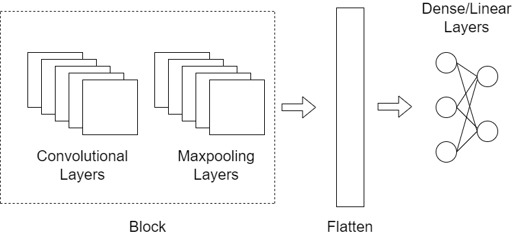
The outputs produced by the first convolutional layers are passed to the next layer. This creates a hierarchical feature extraction process, where low level features of the image are extracted by the initial convolutional layers and the high-level features are tracked by the final/last convolutional layers. Such a stack of convolutions combined with trainable kernels provides CNNs the power to identify objects in images with a great precision, opening the doors of modern computer vision.
The End
I hope this journey through the world of kernels fascinated you towards the concept. Kernels are heavily confused amongst various topics, but their core idea remains the same, which we’ve repeated several times in the blog as neighborhood feature extraction. Instead of using parameters to capture patterns within the data, kernel functions can encode relative proximity of samples to capture trends within the data. But, one must understand that parametric models have their own advantages and their use isn’t obsolete. Most NN models are huge parametric models with millions of parameters and they can solve complex problems such as object detection, image classification, speech synthesis and more.
All images, unless otherwise noted, are by the author.
Kernels: Everything You Need To Know was originally published in Towards Data Science on Medium, where people are continuing the conversation by highlighting and responding to this story.
...