inverse Physics-Informed Neural Net

iPINN ~with code

Solving inverse differential equation problems

(1) Introduction: What is physics-informed?

Many relationships in physics, biology, chemistry, economics, engineering, etc., are defined by differential equations. (Check .) The analytical responses will later be compared to PINN-derived and iPINN-derived responses.

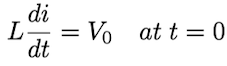
Depending upon the values of the components, this RLC circuit can produce three different types of responses: under-damped, critically damped, and over-damped. All three responses are based on the capacitor charged to a voltage, V₀ , prior to switch closure and the following initial conditions:

(3.1) Under-damped response

An under-damped response occurs when the values of R, L, and C produce the following condition:

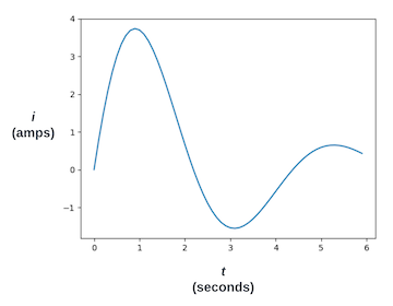
As an example, let R = 1.2 (ohms), L = 1.5 (henries), C = 0.3 (farads), and V₀ = 12 (volts). The analytically-derived response to Equation 2 with these values is:

The following is a plot of the response from Equation 6.

(3.2) Critically damped response

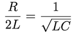
A critically-damped response occurs when the values of R, L, and C produce the following condition:

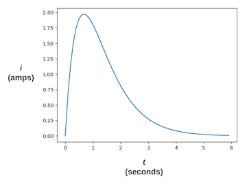
As an example, let R = 4.47 (ohms), L = 1.5 (henries), C = 0.3 (farads), and V₀ = 12 (volts). The analytically-derived response to Equation 2 with these values is:

The following is a plot of the response from Equation 8.

(3.3) Over-damped response

An over-damped response occurs when the values of R, L, and C produce the following condition:

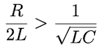
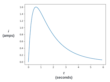
As an example, let R = 6.0 (ohms), L = 1.5 (henries), C = 0.3 (farads), and V₀ = 12 (volts). The analytically-derived response to Equation 2 with these values is:

The following is a plot of the response from Equation 10.

(4) PINN structure

Typically, a neural network is trained with pairs of known input and output data. The training input data is presented to the neural network, and the resulting output is compared to the training output data using a loss function. The loss returned by this function is used via backpropagation to adjust the network’s weights to reduce the loss. PINNs and iPINNs use custom loss functions that include additional loss components for constraining the neural network to produce outputs that comply with the DE being modeled.

A PINN model of the DE in Equation 2 accepts time, t, as input to the neural network and produces a corresponding current, i, as output. Training the PINN to comply with the DE requires both the first and second derivatives of the output with respect to the input, i.e., di/dt and d²i/dt² . These derivatives are available in TensorFlow and PyTorch through each platform’s automatic differentiation function. In this article, the PINN and iPINN are developed with TensorFlow .

(5.1) Neural network model definition

The neural network for the PINN has two fully-connected hidden layers, each with 128 neurons. There is a single input for time points and a single output for the response points.

(5.3) PINN training step

Following is the python code for the training step function. For each training batch, the step function calculates the three components of loss, then uses the total loss to update the weights in the neural network.

loss 1: The initial condition from Equation 3 is compared to the output of the network, pred_y (line 9). The square of the difference is model_loss1 (line 10).

loss 2: The residual (line 30) is calculated at the co-location points. It uses the first-order gradient, dfdx (line 17), and the second-order gradient, dfdx2 (line 26), from GradientTape, along with the output of the network, pred_y (line 29), to calculate the left-hand side of Equation 2. This value squared is model_loss2 (line 31).

loss 3: The initial condition from Equation 4 compares the product of L and the first-order gradient, dfdx (line 17), to v_init2. The square of the difference is model_loss3 (line 19).

The total of the three loss components, model_loss (line 35), is used to calculate the gradients of the loss with respect to the neural network’s weights (line 38). The optimizer then updates the weights (line 41).

The neural network model definition for iPINN is identical to the PINN network (Section 5.1), i.e., two fully-connected hidden layers, each with 128 neurons. There is a single input for time points and a single output for the response points.

(8.1) iPINN initialization

The response of the DE under investigation is loaded in line 4. The two initial conditions (lines 9 and 13) are the same as in the PINN model. As discussed above, R, L, and C are trainable variables in the iPINN model (lines 18–20).

(9) iPINN results

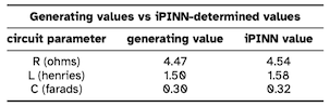
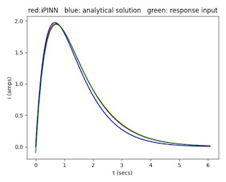
The results of using an iPINN to identify three unknown test responses follow. The test responses presented to the iPINN were generated with the conditions of section 3: under-damped, critically-damped, and over-damped. The tables below compare the R, L, and C component values used to generate the test response to the values determined by the iPINN. Each plot below presents three traces:

• the response curve of the analytical equation (blue)
• the response data (60 points) to be identified by the iPINN (green)
• the output response of the trained iPINN (red)

Under-damped test case:

Critically-damped test case:

Over-damped test case:

(10) Conclusion

This study demonstrates that a neural network can successfully solve differential equations, which describe many relationships in numerous fields of science, engineering, and economics. A physics-informed neural network is trained to solve the second-order differential equation of an electronic circuit resulting in a neural network that produces the same response to an input signal as the actual circuit.

This study also demonstrates that a neural network can determine the parameters of an unknown differential equation. Specifically, an inverse physics-informed neural network is trained to determine the unknown component values of an electronic circuit using only a sample response from the circuit. Further, after determining the unknown component values, the resulting neural network can produce the same response to an input signal as the actual circuit.

Bibliography

[1] M. Raissi, P. Perdikaris, and G. E. Karniadakis, “Physics informed deep learning (part i): Data driven solutions of nonlinear partial differential equations,” 2017. [Online]. Available: https://arxiv.org/abs/1711.10561

[2] M. Raissi, P. Perdikaris, and G. E. Karniadakis, “Physics informed deep learning (part ii): Data-driven discovery of nonlinear partial differential equations,” 2017. [Online]. Available: .

All images, unless otherwise noted, are by the author.

on Medium, where people are continuing the conversation by highlighting and responding to this story.