📚 Hidden Markov Models Explained with a Real Life Example and Python code

Hidden Markov Models are probabilistic models used to solve real life problems ranging from something everyone thinks about at least once a week — how is the weather going to be like tomorrow?[1] — to hard molecular biology problems, such as predicting peptide binders to the human MHC class II molecule[2].

Hidden Markov Models are close relatives of Markov Chains, but their hidden states make them a unique tool to use when you’re interested in determining the probability of a sequence of random variables.

In this article we’ll breakdown Hidden Markov Models into all its different components and see, step by step with both the Math and Python code, which emotional states led to your dog’s results in a training exam. We’ll be using the Viterbi Algorithm to determine the probability of observing a specific sequence of observations, and how you can use the Forward Algorithm to determine the likelihood of an observed sequence, when you’re given a sequence of hidden states.

The real world is full of phenomena for which we can see the final outcome, but can’t actually observe the underlying factors that generated those outcomes. One example is predicting the weather, determining if it’s going to be rainy or sunny tomorrow, based on past weather observations and the observed probabilities of the different weather outcomes.

Although driven by factors we can’t observe, with an Hidden Markov Model it’s possible to model these phenomena as probabilistic systems.

Markov Models with Hidden States

Hidden Markov Models, known as HMM for short, are statistical models that work as a sequence of labeling problems. These are the types of problems that describe the evolution of observable events, which themselves, are dependent on internal factors that can’t be directly observed — they are hidden[3].

An Hidden Markov Model is made of two distinct stochastic processes, meaning those are processes that can be defined as sequences of random variables — variables that depend on random events.

There’s an invisible process and an observable process.

The invisible process is a Markov Chain, like chaining together multiple hidden states that are traversed over time in order to reach an outcome. This is a probabilistic process because all the parameters of the Markov Chain, as well as the score of each sequence, are in fact probabilities[4].

Hidden Markov Models describe the evolution of observable events, which themselves, are dependent on internal factors that can’t be directly observed — they are hidden[3]

Just like any other Markov Chain, in order to know which state you’re going next, the only thing that matters is where you are now — in which state of the Markov Chain you’re currently in. None of the previous history of states you’ve been in the past matters to understand where you’re going next.

This kind of short-term memory is one of the key characteristics of HMMs and it’s called the Markov Assumption, indicating that the probability of reaching the next state is only dependent on the probability of the current state.

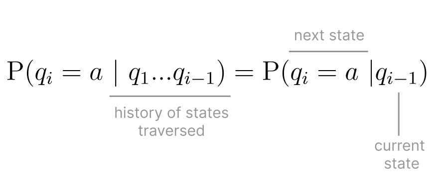
The other key characteristic of an HMM, is that it also assumes that each observation is only dependent on the state that produced it therefore, being completely independent from any other state in the chain[5].

The Markov Assumption states that the probability of reaching the next state is only dependent on the probability of the current state.

This is all great background information on HMM but, what classes of problems are they actually used in?

HMMs help model the behavior of phenomena. Besides modeling and allowing to run simulations, you can also ask different types of questions those phenomena:

• Likelihood or Scoring, as in, determining the probability of observing a sequence
• Decoding the best sequence of states that generated a specific observation
• Learning the parameters of the HMM that led to observing a given sequence, that traversed a specific set of states.

Let's see this in practice!

Dog Training Performance as an HMM

Today you’re not as worried about the weather forecast, what’s on your mind is that your dog is possibly graduating from their training lessons. After all the time, effort and dog treats involved, all you want is for them to succeed.

During dog training sessions, your four-legged friend is expected to do a few actions or tricks, so the trainer can observe and grade their performance. After combining the scores of three trials, they’ll determine if your dog graduates or needs additional training.
The trainer only sees the outcome, but there are several factors involved that can’t be directly observed such as, if your dog is tired, happy, if they don’t like the trainer at all or the other dogs around them.

None of these are directly observed, unless there’s undoubtably a specific action your dog does only when they feel a certain way. Would be great if they could express how they feel in words, maybe in the future!

With Hidden Markov Models fresh in your mind, this looks like the perfect opportunity to try to predict how your dog was feeling during the exam. They might get a certain score because they were feeling tired, maybe they were hungry, or they were annoyed at the trainer.

Your dog has been taking lessons for a while and, based on data collected during that training, you have all the building blocks needed to build a Hidden Markov Model.

In order to build a HMM that models the performance of your dog in the training evaluation you need:

• Hidden States
• Transition Matrix
• Sequence of Observations
• Observation Likelihood Matrix
• Initial Probability Distribution

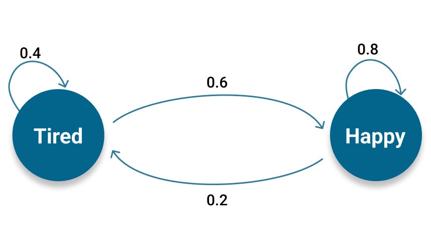
Hidden States are those non-observable factors that influence the observation sequence. You’ll only consider if your dog is Tired or Happy.

Knowing your dog very well, the non-observable factors that can impact their exam performance are simply being tired or happy.

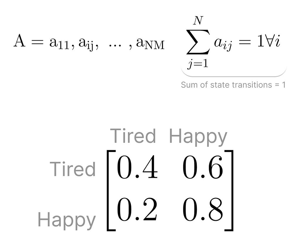
Next you need to know what’s the probability of going from one state to another, which is captured in a Transition Matrix. This matrix must also be row stochastic meaning that the probabilities from one state to any other state in the chain, each row in the matrix, must sum to one.

Regardless of what type of problem you’re solving for, you always need a Sequence of Observations. Each observation representing the result of traversing the Markov Chain. Each observation is drawn from a specific vocabulary.

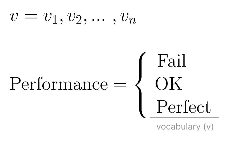
In the case of your dog’s exam you observe the score they get after each trial, which can be Fail, OK or Perfect. These are all the possible terms in the observation vocabulary.

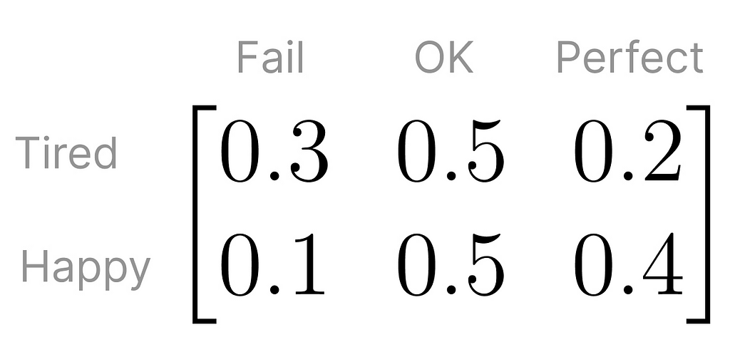
You also need the Observation Likelihood Matrix, which is the probability of an observation being generated from a specific state.

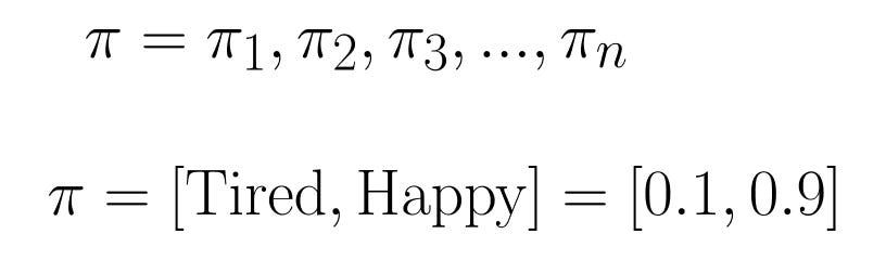
Finally, there’s the Initial Probability Distribution. This is the probability that the Markov Chain will start in each specific hidden state.

There can also be some states will never be the starting state in the Markov Chain. In these situations, their initial probability is zero. And just like the probabilities in the Transition Matrix, these sum of all initial probabilities must add up to one.

The Initial Probability Distribution, along with the Transition Matrix and the Observation Likelihood, make up the parameters of an HMM. These are the probabilities you’re figuring out if you have a sequence of observations and hidden states, and attempt to learn which specific HMM could have generated them.

Putting all of these pieces together, this is what the Hidden Markov model that represents your dog’s performance on the training exam looks like

During the exam, your dog will perform three trials, and graduate only if they don’t Fail in two of those trials.

At the end of the day, if your dog needs more training, you’ll care for them all the same. The big question circling your mind is How are they feeling during the exam.

Imagining a scenario where they graduate with a score of OK — Fail — Perfect exactly in this order, what sequence of emotional states will they be in? Will they be mostly tired, or hungry throughout, or maybe a mix of both?

This type of problem falls right under the category of Decoding problems that HMMs can be applied to. In this case, you’re interested figuring out what’s the best sequence of states that generated a specific sequence of observations, OK — Fail — Perfect.

The problem of decoding the sequence of states that generated a given sequence of observations leverages the Viterbi Algorithm. However, is worth doing a short detour and take a peek into how you could calculate the probability of a given observation sequence — a Likelihood task — using the Forward Algorithm. This will set the stage to better understanding how the Viterbi Algorithm works.

The Forward Algorithm

If you were modeling this problem like a regular Markov Chain, and wanted to calculate the likelihood of observing the sequence of outcomes OK, Fail, Perfect you’d traverse the chain by landing in each specific state that generates the desired outcome. At each step you would take the conditional probability of observing the current outcome given that you’ve observed the previous outcome and multiply that probability by the transition probability of going from one state to the other.

The big difference is that, in a regular Markov Chain, all states are well known and observable. Not in an Hidden Markov Model! In an Hidden Markov Model you observe a sequence of outcomes, not knowing which specific sequence of hidden states had to be traversed in order to observe that.

The big difference is that, in a regular Markov Chain, all states are well known and observable. Not in an Hidden Markov Model!

At this point you might be thinking, Well I can simply traverse all possible paths and eventually have a rule to pick between equivalent paths. The mathematical definition for this approach looks something like this

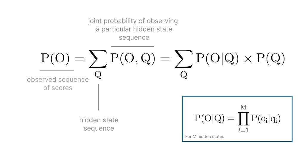
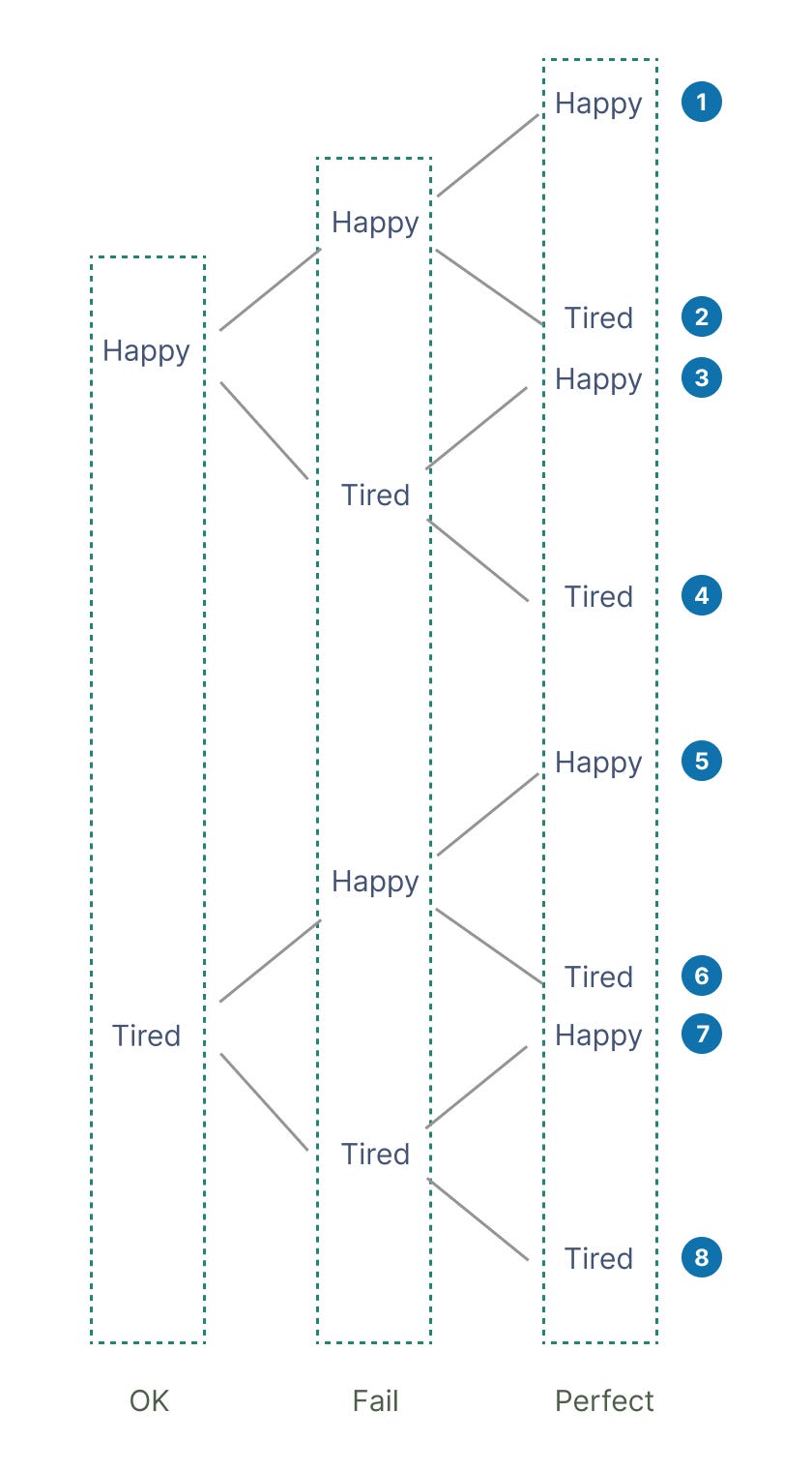
That’s one strategy for sure! You’d have to calculate the probability of observing the sequence OK, Fail, Perfect for every single combination of hidden states that could ever generate that sequence.

When you have a small enough number of hidden states and sequence of observed outcomes, it's possible to do that calculation within a reasonable time.

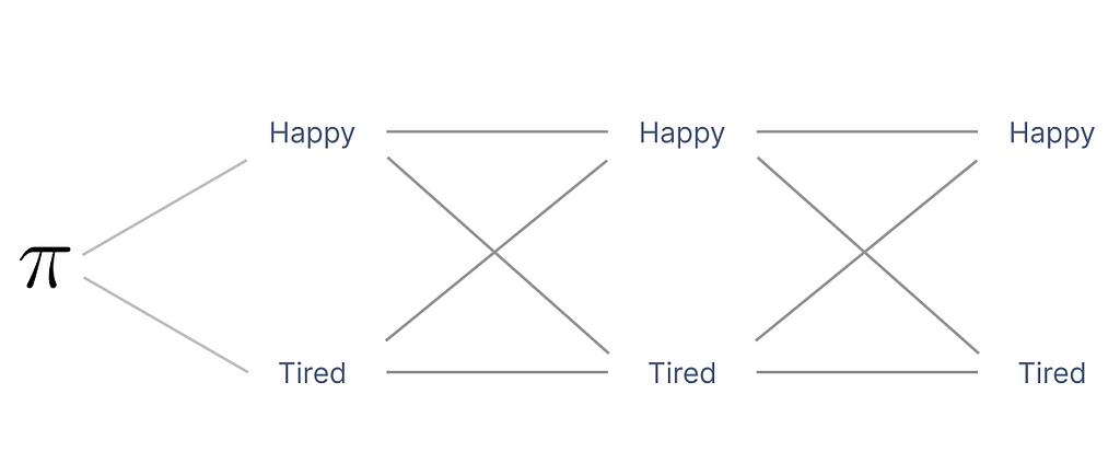
Thankfully, the Hidden Markov model you just defined is relatively simple, with 3 observed outcomes and 2 hidden states.

For an observed sequence of length L outcomes, on a HMM with M hidden states, you have “M to the power L” possible states which in your case, means 2 to the power of 3, i.e., 8 possible paths for the sequence OK — Fail — Perfect, involving an exponential computational complexity of O(M^L L), described in Big O-Notation. As the complexity of the model increases, the number of paths you need to take into account grows exponentially.

As the complexity of the model increases, the number of paths you need to take into account grows exponentially.

This is where the Forward Algorithm shines.

The Forward Algorithm calculates the probability of a new symbol in the observed sequence, without the need to calculate the probabilities of all possible paths that form that sequence [3].

Instead of computing the probabilities of all possible paths that form that sequence the algorithm defines the forward variable and calculates its value recursively.

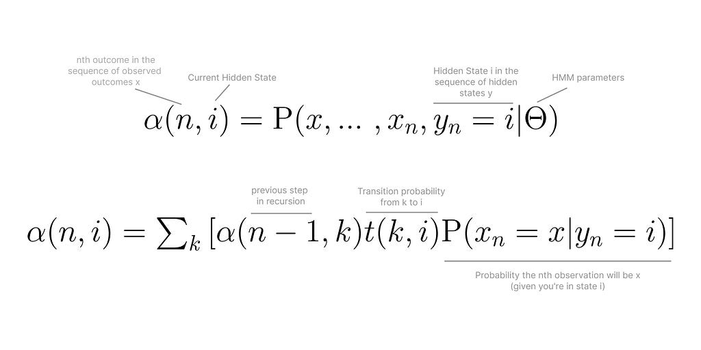
The fact that it uses recursion, is the key reason why this algorithm is faster than calculating all the probabilities of possible paths. In fact, it can calculate the probability of observing the sequence x in only “L times M squared” computations, instead of “M to the power of L times L”.

In your case, with 2 hidden states and a sequence of 3 observed outcomes, it’s the difference between calculating the probabilities O(MˆL L) = 2³x3 = 8x3 = 24 times, as opposed to O(L Mˆ2)=3*2²=3x4 = 12 times.

This reduction in the number of calculations is achieved by Dynamic Programming, a programming technique that uses an auxiliary data structures to store intermediate information, therefore making sure the same calculations are not done multiple times.

Every time the algorithm is about to calculate a new probability it checks if it has already computed it, and if so, it can easily access that value in the intermediate data structure. Otherwise, the probability is calculated and the value is stored.

Let’s get back to your decoding problem, using the Viterbi Algorithm.

The Viterbi Algorithm

Thinking in pseudo code, If you were to brute force your way into decoding the sequence of hidden states that generate a specific observation sequence, all you needed to do was:

• generate all possible permutations of paths that lead to the desired observation sequence
• use the Forward Algorithm to calculate the likelihood of each observation sequence, for each possible sequence of hidden states
• pick the sequence of hidden states with highest probability

For your specific HMM, there are 8 possible paths that lead to an outcome of OK — Fail — Perfect. Add just one more observation, and you’ll have double the amount of possible sequences of hidden states! Similarly to what was described for the Forward Algorithm, you easily end up with an exponentially complex algorithm and hit performance ceiling.

The Viterbi Algorithm, gives you a hand with that.

When the sequence of hidden states in the HMM is traversed, at each step, the probability vt(j) is the probability that the HMM is in the hidden state j after seeing the observation and is being traversed through the most probable state that lead to j.

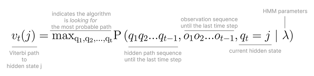
The key to decoding the sequence of hidden states that generate a specific observation sequence, is this concept of the most probable path. Also called the Viterbi path, the most probable path, is the path that has highest likelihood, from all the paths that can lead to any given hidden state.

The key to decoding the sequence of hidden states that generate a specific observation sequence, is to use the Viterbi path. The most probable path that leads to any given hidden state.

You can draw a parallel between the Forward Algorithm and the Viterbi Algorithm. Where the Forward Algorithm sums all probabilities to obtain the likelihood of reaching a certain state taking into account all the paths that lead there, the Viterbi algorithm doesn’t want to explore all possibilities. It focuses on the most probable path that leads to any given state.

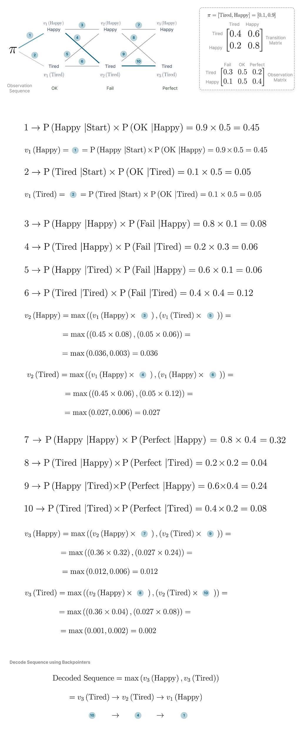
Going back to the task of decoding the sequence of hidden states that lead to the scores of OK — Fail — Perfect in their exam, running the Viterbi Algorithm by hand would look like this

Another unique characteristic of the Viterbi algorithm is that it must have a way to keep track of all the paths that led to any given hidden state, in order to compare their probabilities. To do that it keeps track of backpointers to each hidden state, using an auxiliary data structure typical of dynamic programming algorithms. That way it can easily access the probability of any viterbi path traversed in the past.

Backpointers are the key to figure out the most probable path that leads to an observation sequence.

In the example of your dogs’ exam, when you calculate the Viterbi paths v3(Happy) and v3(Tired), you pick the path with highest probability and start going backwards, i.e., backtracking, through all the paths that led to where you are.

The Viterbi Algorithm in Python

Doing all of this by hand is time consuming and error prone. Miss one significant digit and you might have to start from scratch and re-check all your probabilities!

The good news is that you can leverage software libraries like hmmlearn, and with a few lines of code you can decode the sequence of hidden states that lead to your dog graduating with OK — Fail — Perfect in the trials, exactly in this order.

from hmmlearn import hmm
import numpy as np

## Part 1. Generating a HMM with specific parameters and simulating the exam
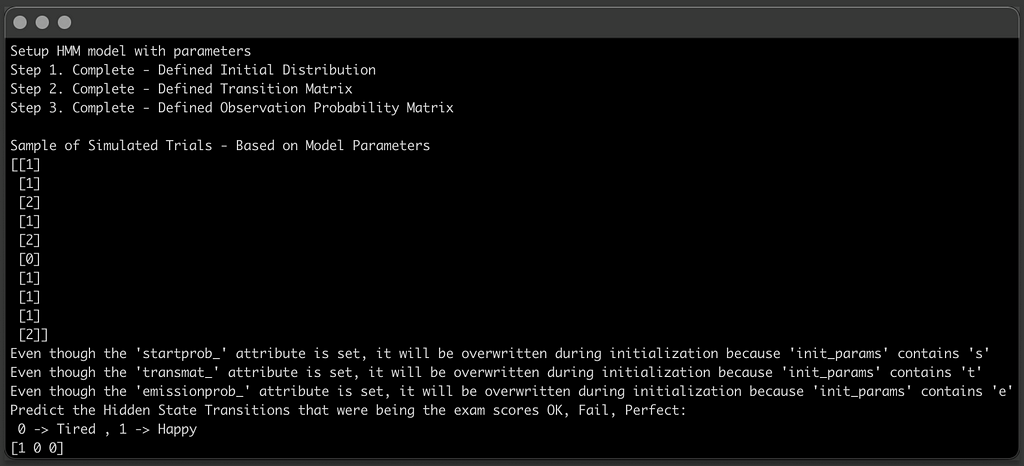
print("Setup HMM model with parameters")
# init_params are the parameters used to initialize the model for training
# s -> start probability
# t -> transition probabilities
# e -> emission probabilities
model = hmm.CategoricalHMM(n_components=2, random_state=425, init_params='ste')

# initial probabilities
# probability of starting in the Tired state = 0
# probability of starting in the Happy state = 1
initial_distribution = np.array([0.1, 0.9])
model.startprob_ = initial_distribution

print("Step 1. Complete - Defined Initial Distribution")

# transition probabilities
#        tired    happy
# tired   0.4      0.6
# happy   0.2      0.8

transition_distribution = np.array([[0.4, 0.6], [0.2, 0.8]])
model.transmat_ = transition_distribution
print("Step 2. Complete - Defined Transition Matrix")

# observation probabilities
#        Fail    OK      Perfect
# tired   0.3    0.5       0.2
# happy   0.1    0.5       0.4

observation_probability_matrix = np.array([[0.3, 0.5, 0.2], [0.1, 0.5, 0.4]])
model.emissionprob_ = observation_probability_matrix
print("Step 3. Complete - Defined Observation Probability Matrix")

# simulate performing 100,000 trials, i.e., aptitude tests
trials, simulated_states = model.sample(100000)

# Output a sample of the simulated trials
# 0 -> Fail
# 1 -> OK
# 2 -> Perfect
print("\nSample of Simulated Trials - Based on Model Parameters")
print(trials[:10])

## Part 2 - Decoding the hidden state sequence that leads
## to an observation sequence of OK - Fail - Perfect

# split our data into training and test sets (50/50 split)
X_train = trials[:trials.shape[0] // 2]
X_test = trials[trials.shape[0] // 2:]

model.fit(X_train)

# the exam had 3 trials and your dog had the following score: OK, Fail, Perfect (1, 0 , 2)
exam_observations = [[1, 0, 2]]
predicted_states = model.predict(X=[[1, 0, 2]])
print("Predict the Hidden State Transitions that were being the exam scores OK, Fail, Perfect: \n 0 -> Tired , "
      "1 -> Happy")
print(predicted_states)

In a few seconds you get an output that matches results the calculations you did by hand, much fast and with much less room for error.

Conclusion

What’s fascinating about Hidden Markov Models is how this statistical tool created in the mid 1960’s [6] is so powerful and applicable to real world problems in such distinct areas, from weather forecasting to finding the next word in a sentence.

In this article, you had the chance to learn about the different components of an HMM, how they can be applied to different types of tasks, and spotting the similarities between the Forward Algorithm and Viterbi Algorithm. Two very similar algorithms that use dynamic programming to deal with the exponential number of calculations involved.

Either doing the calculations by hand or plugging in the parameters into TensorFlow code, hope you enjoyed diving deep into the world of HMMs.

Thank you for reading!

References

1. D. Khiatani and U. Ghose, “Weather forecasting using Hidden Markov Model,” 2017 International Conference on Computing and Communication Technologies for Smart Nation (IC3TSN), Gurgaon, India, 2017, pp. 220–225, doi: 10.1109/IC3TSN.2017.8284480.
2. Noguchi H, Kato R, Hanai T, Matsubara Y, Honda H, Brusic V, Kobayashi T. Hidden Markov model-based prediction of antigenic peptides that interact with MHC class II molecules. J Biosci Bioeng. 2002;94(3):264–70. doi: 10.1263/jbb.94.264. PMID: 16233301.
3. Yoon BJ. Hidden Markov Models and their Applications in Biological Sequence Analysis. Curr Genomics. 2009 Sep;10(6):402–15. doi: 10.2174/138920209789177575. PMID: 20190955; PMCID: PMC2766791.
4. Eddy, S. What is a hidden Markov model?. Nat Biotechnol 22, 1315–1316 (2004). https://doi.org/10.1038/nbt1004-1315
5. Jurafsky, Dan and Martin, James H.. Speech and language processing : an introduction to natural language processing, computational linguistics, and speech recognition. Upper Saddle River, N.J.: Pearson Prentice Hall, 2009.
6. Baum, Leonard E., and Ted Petrie. “Statistical Inference for Probabilistic Functions of Finite State Markov Chains.” The Annals of Mathematical Statistics 37, no. 6 (1966): 1554–63.

Hidden Markov Models Explained with a Real Life Example and Python code was originally published in Towards Data Science on Medium, where people are continuing the conversation by highlighting and responding to this story.