📚 A Gentle Introduction to Deep Reinforcement Learning in JAX

Solving the CartPole environment with DQN in under a second

Recent progress in Reinforcement Learning (RL), such as Waymo’s autonomous taxis or DeepMind’s superhuman chess-playing agents, complement classical RL with Deep Learning components such as Neural Networks and Gradient Optimization methods.

Building on the foundations and coding principles introduced in one of my previous stories, we’ll discover and learn to implement Deep Q-Networks (DQN) and replay buffers to solve OpenAI’s CartPole environment. All of that in under a second using JAX!

For an introduction to JAX, vectorized environments, and Q-learning, please refer to the content of this story:

Vectorize and Parallelize RL Environments with JAX: Q-learning at the Speed of Light⚡

Our framework of choice for deep learning will be DeepMind’s Haiku library, which I recently introduced in the context of Transformers:

Implementing a Transformer Encoder from Scratch with JAX and Haiku 🤖

This article will cover the following sections:

• Why do we need Deep RL?
• Deep Q-Networks, theory and practice
• Replay Buffers
• Translating the CartPole environment to JAX
• The JAX way to write efficient training loops

As always, all the code presented in this article is available on GitHub:

GitHub - RPegoud/jym: JAX implementation of RL algorithms and vectorized environments

Why do we need Deep RL?

In previous articles, we introduced Temporal Difference Learning algorithms and in particular Q-learning.

Simply put, Q-learning is an off-policy algorithm (the target policy is not the policy used for decision-making) maintaining and updating a Q-table, an explicit mapping of states to corresponding action values.

While Q-learning is a practical solution for environments with discrete action spaces and restricted observation spaces, it struggles to scale well to more complex environments. Indeed, creating a Q-table requires defining the action and observation spaces.

Consider the example of autonomous driving, the observation space is composed of an infinity of potential configurations derived from camera feeds and other sensory inputs. On the other hand, the action space includes a wide spectrum of steering wheel positions and varying levels of force applied to the brake and accelerator.

Even though we could theoretically discretize the action space, the sheer volume of possible states and actions leads to an impractical Q-table in real-world applications.

Finding optimal actions in large and complex state-action spaces thus requires powerful function approximation algorithms, which is precisely what Neural Networks are. In the case of Deep Reinforcement Learning, neural nets are used as a replacement for the Q-table and provide an efficient solution to the curse of dimensionality introduced by large state spaces. Furthermore, we do not need to explicitly define the observation space.

Deep Q-Networks & Replay Buffers

DQN uses two types of neural networks in parallel, starting with the “online” network which is used for Q-value prediction and decision-making. On the other hand, the “target” network is used to create stable Q-targets to assess the performance of the online net via the loss function.

Similarly to Q-learning, DQN agents are defined by two functions: act and update.

Act

The act function implements an epsilon-greedy policy with respect to Q-values, which are estimated by the online neural network. In other words, the agent selects the action corresponding to the maximum predicted Q-value for a given state, with a set probability of acting randomly.

You might remember that Q-learning updates its Q-table after every step, however, in Deep Learning it is common practice to compute updates using gradient descent on a batch of inputs.

For this reason, DQN stores experiences (tuples containing state, action, reward, next_state, done_flag) in a replay buffer. To train the network, we’ll sample a batch of experiences from this buffer instead of using only the last experience (more details in the Replay Buffer section).

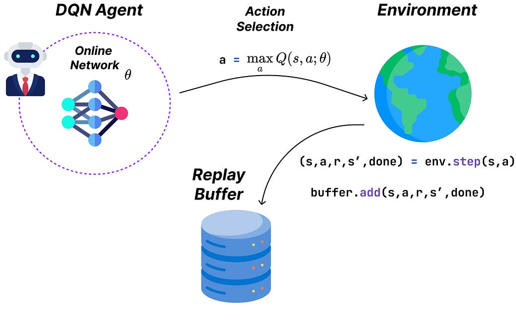
Here’s a JAX implementation of the action-selection part of DQN:

The only subtlety of this snippet is that the model attribute doesn’t contain any internal parameters as is usually the case in frameworks such as PyTorch or TensorFlow.

Here, the model is a function representing a forward pass through our architecture, but the mutable weights are stored externally and passed as arguments. This explains why we can use jit while passing the self argument as static (the model being stateless as other class attributes).

Update

The update function is responsible for training the network. It computes a mean squared error (MSE) loss based on the temporal-difference (TD) error:

In this loss function, θ denotes the parameters of the online network, and θ− represents the parameters of the target network. The parameters of the target network are set on the online network’s parameters every N steps, similar to a checkpoint (N is a hyperparameter).

This separation of parameters (with θ for the current Q-values and θ− for the target Q-values) is crucial to stabilize training.

Using the same parameters for both would be similar to aiming at a moving target, as updates to the network would immediately shift the target values. By periodically updating θ− (i.e. freezing these parameters for a set number of steps), we ensure stable Q-targets while the online network continues to learn.

Finally, the (1-done) term adjusts the target for terminal states. Indeed, when an episode ends (i.e. ‘done’ is equal to 1), there is no next state. Therefore, the Q-value for the next state is set to 0.

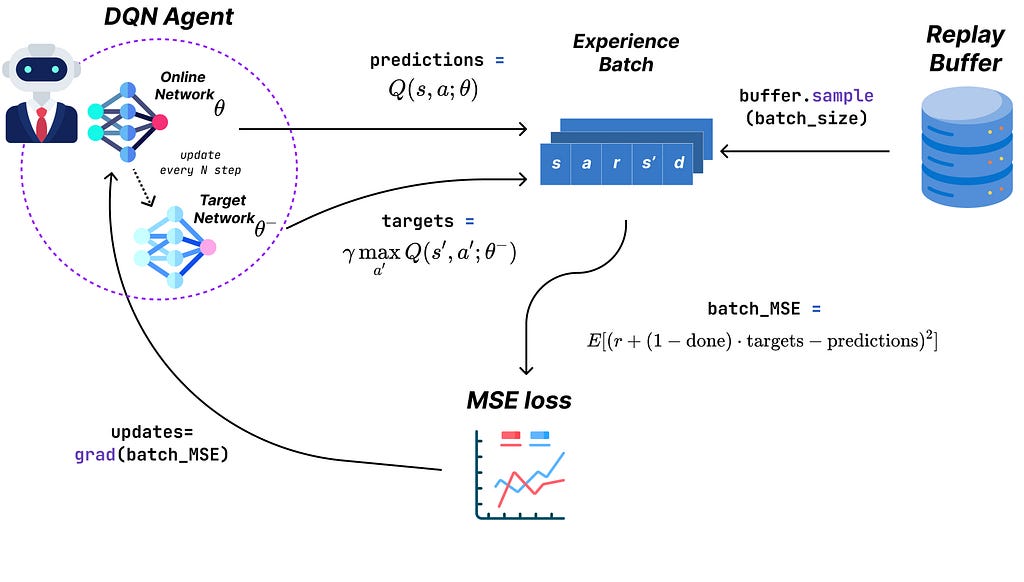
Implementing the update function for DQN is slightly more complex, let’s break it down:

• First, the _loss_fn function implements the squared error described previously for a single experience.
• Then, _batch_loss_fn acts as a wrapper for _loss_fn and decorates it with vmap, applying the loss function to a batch of experiences. We then return the average error for this batch.
• Finally, update acts as a final layer to our loss function, computing its gradient with respect to the online network parameters, the target network parameters, and a batch of experiences. We then use Optax (a JAX library commonly used for optimization) to perform an optimizer step and update the online parameters.

Notice that, similarly to the replay buffer, the model and optimizer are pure functions modifying an external state. The following line serves as a good illustration of this principle:

updates, optimizer_state = optimizer.update(grads, optimizer_state)

This also explains why we can use a single model for both the online and target networks, as the parameters are stored and updated externally.

# target network predictions
self.model.apply(target_net_params, None, state)
# online network predictions
self.model.apply(online_net_params, None, state)

For context, the model we use in this article is a multi-layer perceptron defined as follows:

N_ACTIONS = 2
NEURONS_PER_LAYER = [64, 64, 64, N_ACTIONS]
online_key, target_key = vmap(random.PRNGKey)(jnp.arange(2) + RANDOM_SEED)

@hk.transform
def model(x):
    # simple multi-layer perceptron
    mlp = hk.nets.MLP(output_sizes=NEURONS_PER_LAYER)
    return mlp(x)

online_net_params = model.init(online_key, jnp.zeros((STATE_SHAPE,)))
target_net_params = model.init(target_key, jnp.zeros((STATE_SHAPE,)))

prediction = model.apply(online_net_params, None, state)

Replay Buffer

Now let us take a step back and look closer at replay buffers. They are widely used in reinforcement learning for a variety of reasons:

• Generalization: By sampling from the replay buffer, we break the correlation between consecutive experiences by mixing up their order. This way, we avoid overfitting to specific sequences of experiences.
• Diversity: As the sampling is not limited to recent experiences, we generally observe a lower variance in updates and prevent overfitting to the latest experiences.
• Increased sample efficiency: Each experience can be sampled multiple times from the buffer, enabling the model to learn more from individual experiences.

Finally, we can use several sampling schemes for our replay buffer:

• Uniform sampling: Experiences are sampled uniformly at random. This type of sampling is straightforward to implement and allows the model to learn from experiences independently from the timestep they were collected.
• Prioritized sampling: This category includes different algorithms such as Prioritized Experience Replay (“PER”, Schaul et al. 2015) or Gradient Experience Replay (“GER”, Lahire et al., 2022). These methods attempt to prioritize the selection of experiences according to some metric related to their “learning potential” (the amplitude of the TD error for PER and the norm of the experience’s gradient for GER).

For the sake of simplicity, we’ll implement a uniform replay buffer in this article. However, I plan to cover prioritized sampling extensively in the future.

As promised, the uniform replay buffer is quite easy to implement, however, there are a few complexities related to the use of JAX and functional programming. As always, we have to work with pure functions that are devoid of side effects. In other words, we are not allowed to define the buffer as a class instance with a variable internal state.

Instead, we initialize a buffer_state dictionary that maps keys to empty arrays with predefined shapes, as JAX requires constant-sized arrays when jit-compiling code to XLA.

buffer_state = {
    "states": jnp.empty((BUFFER_SIZE, STATE_SHAPE), dtype=jnp.float32),
    "actions": jnp.empty((BUFFER_SIZE,), dtype=jnp.int32),
    "rewards": jnp.empty((BUFFER_SIZE,), dtype=jnp.int32),
    "next_states": jnp.empty((BUFFER_SIZE, STATE_SHAPE), dtype=jnp.float32),
    "dones": jnp.empty((BUFFER_SIZE,), dtype=jnp.bool_),
}

We will use a UniformReplayBuffer class to interact with the buffer state. This class has two methods:

• add: Unwraps an experience tuple and maps its components to a specific index. idx = idx % self.buffer_size ensures that when the buffer is full, adding new experiences overwrites older ones.
• sample: Samples a sequence of random indexes from the uniform random distribution. The sequence length is set by batch_size while the range of the indexes is [0, current_buffer_size-1]. This ensures that we do not sample empty arrays while the buffer is not yet full. Finally, we use JAX’s vmap in combination with tree_map to return a batch of experiences.

Translating the CartPole environment to JAX

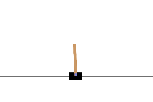
Now that our DQN agent is ready for training, we’ll quickly implement a vectorized CartPole environment using the same framework as introduced in an earlier article. CartPole is a control environment having a large continuous observation space, which makes it relevant to test our DQN.

The process is quite straightforward, we reuse most of OpenAI’s Gymnasium implementation while making sure we use JAX arrays and lax control flow instead of Python or Numpy alternatives, for instance:

# Python implementation
force = self.force_mag if action == 1 else -self.force_mag
# Jax implementation
force = lax.select(jnp.all(action) == 1, self.force_mag, -self.force_mag)            )

# Python
costheta, sintheta = math.cos(theta), math.sin(theta)
# Jax
cos_theta, sin_theta = jnp.cos(theta), jnp.sin(theta)

# Python
if not terminated:
  reward = 1.0
...
else: 
  reward = 0.0
# Jax
reward = jnp.float32(jnp.invert(done))

For the sake of brevity, the full environment code is available here:

jym/src/envs/control/cartpole.py at main · RPegoud/jym

The JAX way to write efficient training loops

The last part of our implementation of DQN is the training loop (also called rollout). As mentioned in previous articles, we have to respect a specific format in order to take advantage of JAX’s speed.

The rollout function might appear daunting at first, but most of its complexity is purely syntactic as we’ve already covered most of the building blocks. Here’s a pseudo-code walkthrough:

1. Initialization:
  * Create empty arrays that will store the states, actions, rewards 
    and done flags for each timestep. Initialize the networks and optimizer
    with dummy arrays.
  * Wrap all the initialized objects in a val tuple

2. Training loop (repeat for i steps):
  * Unpack the val tuple
  * (Optional) Decay epsilon using a decay function
  * Take an action depending on the state and model parameters
  * Perform an environment step and observe the next state, reward 
    and done flag
  * Create an experience tuple (state, action, reward, new_state, done)
    and add it to the replay buffer
  * Sample a batch of experiences depending on the current buffer size
    (i.e. sample only from experiences that have non-zero values)
  * Update the model parameters using experience batch
  * Every N steps, update the target network's weights 
    (set target_params = online_params)
  * Store the experience's values for the current episode and return 
    the updated `val` tuple

We can now run DQN for 20,000 steps and observe the performances. After around 45 episodes, the agent manages to obtain decent performances, balancing the pole for more than 100 steps consistently.

The green bars indicate that the agent managed to balance the pole for more than 200 steps, solving the environment. Notably, the agent set its record on the 51st episode, with 393 steps.

The 20.000 training steps were executed in just over a second, at a rate of 15.807 steps per second (on a single CPU)!

These performances hint at JAX’s impressive scaling capabilities, allowing practitioners to run large-scale parallelized experiments with minimal hardware requirements.

Running for 20,000 iterations: 100%|██████████| 20000/20000 [00:01<00:00, 15807.81it/s]

We’ll take a closer look at parallelized rollout procedures to run statistically significant experiments and hyperparameter searches in a future article!

In the meantime, feel free to reproduce the experiment and dabble with hyperparameters using this notebook:

jym/notebooks/control/cartpole/dqn_cartpole.ipynb at main · RPegoud/jym

Conclusion

As always, thanks for reading this far! I hope this article provided a decent introduction to Deep RL in JAX. Should you have any questions or feedback related to the content of this article, make sure to let me know, I’m always happy to have a little chat ;)

Until next time 👋

Credits:

• Cartpole Gif, OpenAI Gymnasium library, (MIT license)

A Gentle Introduction to Deep Reinforcement Learning in JAX was originally published in Towards Data Science on Medium, where people are continuing the conversation by highlighting and responding to this story.