Object detection using the power and simplicity of the KerasCV library.

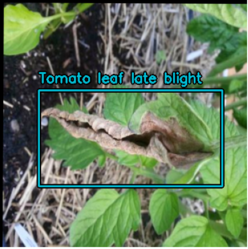
The blue box is referred to as a bounding box and the class name is placed right above it. Object detection can thus be broken down into two mini-problems:
- A regression problem where the model must predict x and y coordinates for the both the upper left corner and the lower right corner of the box.
- A classification problem where the model must predict what class of object the box is observing.
In this example, the bounding box was created and labeled by a human. We would like to automate this process, and a well-trained object detection model can do just that.
I sat down to review my study material regarding object detection, and was promptly disappointed. Unfortunately, most introductory material scarcely mention object detection. François Chollet in Deep Learning with Python [1] states:
Note that we won’t cover object detection, because it would be too specialized and too complicated for an introductory book.
Aurélion Géron [2] provides a lot of textual content covering the ideas behind object detection, but provides only a few lines of code covering an object detection task with dummy bounding boxes, far from the end-to-end pipeline I was looking for. Andrew Ng’s [3] famous Deep Learning Specialization course goes the deepest on object detection, but even he ends the coding lab by loading a pre-trained object detection model and just doing inference.
Looking to go deeper, I started to sketch out the outline of an object detection pipeline. Just to do pre-processing for a RetinaNet model, one would have to do the following (note: other object detection models such as YOLO would require different steps):
- Take input images and resize them all to be the same size, with padding to prevent the aspect ratio from getting messed up. Oh, don’t forget about the bounding boxes; these also need to be appropriately reshaped or you will ruin your data.
- Generate anchor boxes at different scales and aspect ratios based on the ground truth bounding boxes in the training set. These anchor boxes act as reference points for the model during training.
- Assign labels to the anchor boxes based on their overlap with ground truth boxes. Anchor boxes with high overlap are labeled as positive examples, while those with low overlap are labeled as negative examples.
- There are multiple ways to describe the same bounding box. You would need to implement functions for converting between these different formats. More on this in a moment.
- Implement data augmentation, taking care to not only augment the images but also the boxes. In theory you can omit this, but in practice this is necessary to help our models generalize well.
. As I read the documentation, it began to dawn on me that this is the future of computer vision in TensorFlow/Keras. From their introduction:
KerasCV can be understood as a horizontal extension of the Keras API: the components are new first-party Keras objects that are too specialized to be added to core Keras. They receive the same level of polish and backwards compatibility guarantees as the core Keras API, and they are maintained by the Keras team.
“But why did none of my study materials even mention this?” I wondered. The answer is simple: this is a fairly new library. The first commit on GitHub was on April 13th, 2022, too new to show up even in the latest editions of my textbooks. In fact, the 1.0 version of the library hasn’t even been released yet (as of November 10th, 2023 it is on 0.6.4). I expect KerasCV will be discussed in detail by the next editions of my textbooks and online courses (to be fair, Gèron does mention in passing a “new Keras NLP project” and Keras CV project that the reader may be interested in).
Being so new, KerasCV doesn’t have many tutorials aside from those published by the Keras team themselves (. In addition, the documentation is lacking in some areas (I’m looking at you, MultiClassNonMaxSuppression). As you play around with KerasCV, try not to be discouraged by these issues. In fact, this is a great opportunity to become a contributor to the KerasCV codebase!
This tutorial will focus on implementation details of KerasCV. I will briefly review some high-level concepts in object detection, but I will assume the reader has some background knowledge on concepts such as the RetinaNet architecture. The code shown here has been edited and rearranged for clarity, please see the Kaggle notebook linked above for the complete code.
Finally, a note on safety. The model created here is not intended to be state-of-the-art; treat this as a high-level tutorial. Further fine-tuning and data cleaning would be expected before this plant disease detection model could be implemented in production. It would be a good idea to run any predictions a model makes by a human expert to confirm a diagnosis.
Inspecting the Data
The PlantDoc dataset contains 2,569 images across 13 plant species and 30 classes. The goal of the dataset is set out in the abstract of the paper PlantDoc: A Dataset for Visual Plant Disease Detection by Singh et. al [4].
India loses 35% of the annual crop yield due to plant diseases. Early detection of plant diseases remains difficult due to the lack of lab infrastructure and expertise. In this paper, we explore the possibility of computer vision approaches for scalable and early plant disease detection.
This is a noble goal, and an area where computer vision can do a lot of good for farmers.
Roboflow allows us to download the dataset in a variety of different formats. Since we are using TensorFlow, let’s download the dataset as a TFRecord. A TFRecord is a specific format used in TensorFlow that is designed to store large amounts of data efficiently. The data is represented by a sequence of records, where each record is a key-value pair. Each key is a referred to as a feature. The downloaded zip file contains four files, two for training and two for validation:
- leaves_label_map.pbtxt : This is a Protocol Buffers text format file, which is used to describe the structure of the data. Opening the file in a text editor, I see that there are thirty classes. There are a mixture of healthy leaves such as Apple leaf and unhealthy leaves such as Apple Scab Leaf .
- leaves.tfrecord : This is the TFRecord file that contains all of our data.
Our first step is to inspect leaves.tfrecord. What features do our records contain? Unfortunately this is not specified by Roboflow.
train_tfrecord_file = '/kaggle/input/plants-dataset/leaves.tfrecord'
val_tfrecord_file = '/kaggle/input/plants-dataset/test_leaves.tfrecord'

# Create a TFRecordDataset
train_dataset = tf.data.TFRecordDataset([train_tfrecord_file])
val_dataset = tf.data.TFRecordDataset([val_tfrecord_file])

# Iterate over a few entries and print their content. Uncomment this to look at the raw data
for record in train_dataset.take(1):
  example = tf.train.Example()
  example.ParseFromString(record.numpy())
  print(example)
I see the following features printed:
- image/encoded : This is the encoded binary representation of an image. In the case of this dataset the images are encoded in the jpeg format.
- image/height : This is the height of each image.
- image/width : This is the width of each image.
- image/object/bbox/xmin : This is the x-coordinate of the top-left corner of our bounding box.
- image/object/bbox/xmax : This is the x-coordinate of the bottom-right corner of our bounding box.
- image/object/bbox/ymin : This is the y-coordinate of the top-left corner of our bounding box.
- image/object/bbox/ymax : This is the y-coordinate of the bottom-right corner of our bounding box.
- image/object/class/label : These are the labels associated with each bounding box.
Now we want to take all of the images and associated bounding boxes and put them together in a TensorFlow Dataset object. Dataset objects allow you to store large amounts of data without overwhelming your system’s memory. This is accomplished through features such as lazy loading and batching. Lazy loading means that the data is not loaded into memory until its explicitly requested (for example when performing transformations or during training). Batching means that only a select number of images (usually 8, 16, 32, etc.) get loaded into memory at once. In short, I recommend always converting your data into Dataset objects, especially when you are dealing with large amounts of data (typical in object detection).
To convert a TFRecord to a Dataset object in TensorFlow, you can use the tf.data.TFRecordDataset class to create a dataset from our TFRecord file, and then apply parsing functions using the map method to extract and preprocess features. The parsing code is shown below.
def parse_tfrecord_fn(example):
    feature_description = {
        'image/encoded': tf.io.FixedLenFeature([], tf.string),
        'image/height': tf.io.FixedLenFeature([], tf.int64),
        'image/width': tf.io.FixedLenFeature([], tf.int64),
        'image/object/bbox/xmin': tf.io.VarLenFeature(tf.float32),
        'image/object/bbox/xmax': tf.io.VarLenFeature(tf.float32),
        'image/object/bbox/ymin': tf.io.VarLenFeature(tf.float32),
        'image/object/bbox/ymax': tf.io.VarLenFeature(tf.float32),
        'image/object/class/label': tf.io.VarLenFeature(tf.int64),
    }

    parsed_example = tf.io.parse_single_example(example, feature_description)

    # Decode the JPEG image and normalize the pixel values to the [0, 1] range.
    img = tf.image.decode_jpeg(parsed_example['image/encoded'], channels=3) # Returned as uint8
    # Normalize the pixel values to [0, 256]
    img = tf.image.convert_image_dtype(img, tf.uint8)

    # Get the bounding box coordinates and class labels.
    xmin = tf.sparse.to_dense(parsed_example['image/object/bbox/xmin'])
    xmax = tf.sparse.to_dense(parsed_example['image/object/bbox/xmax'])
    ymin = tf.sparse.to_dense(parsed_example['image/object/bbox/ymin'])
    ymax = tf.sparse.to_dense(parsed_example['image/object/bbox/ymax'])
    labels = tf.sparse.to_dense(parsed_example['image/object/class/label'])

    # Stack the bounding box coordinates to create a [num_boxes, 4] tensor.
    rel_boxes = tf.stack([xmin, ymin, xmax, ymax], axis=-1)
    boxes = keras_cv.bounding_box.convert_format(rel_boxes, source='rel_xyxy', target='xyxy', images=img)

    # Create the final dictionary.
    image_dataset = {
        'images': img,
        'bounding_boxes': {
            'classes': labels,
            'boxes': boxes
        }
    }
    return image_dataset
Let’s break this down:
- feature_description : This is a dictionary that describes the expected format of each of our features. We use tf.io.FixedLenFeature when the length of a feature is fixed across all examples in the dataset, and tf.io.VarLenFeature when some variability in the length is expected. Since the number of bounding boxes is not constant across our dataset (some images have more boxes, others have less), we use tf.io.VarLenFeature for anything related to bounding boxes.
- We decode the image files using tf.image.decode_jpeg , since our images are encoded in the JPEG format.
- Note the use of tf.sparse.to_dense used for the bounding box coordinates and labels. When we use tf.io.VarLenFeature the information comes back as a sparse matrix. A sparse matrix is a matrix in which most of the elements are zero, resulting in a data structure that efficiently stores only the non-zero values along with their indices. Unfortunately, many pre-processing functions in TensorFlow require dense matrices. This includes tf.stack , which we use to horizontally stack information from multiple bounding boxes together. To fix this issue, we use tf.sparse.to_dense to convert the sparse matrices to dense matrices.
- After stacking the boxes, we use KerasCV’s keras_cv.bounding_box.convert_format function. When inspecting the data, I noticed that the bounding box coordinates were normalized between 0 and 1. This means that the numbers represent percentages of the images total width/height. So a value of 0.5 represents 50% * image_width, as an example. This is a relative format, which Keras refers to as REL_XYXY , rather than the absolute format XYXY. In theory converting to the absolute format is not necessary, but I was running into bugs when training my model with relative coordinates. See the . We are only using YOLO only as a feature extractor, not as an object detector.
- Feature pyramid network (FPN). This is a model architecture that generates a “pyramid” of feature maps at different scales to detect objects of various sizes. It does this by combining low-resolution, semantically strong features with high-resolution, semantically weak features via a top-down pathway and lateral connections. Take a look at [5] that introduced the FPN.
- Two task-specific subnetworks. These subnetworks take each level of the pyramid and detects objects in each. One subnetwork identifies classes (classification) while the other identifies bounding boxes (regression). These subnetworks are untrained.
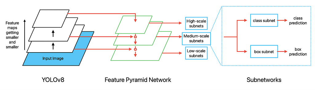
Earlier we resized the images to be of size 416 by 416. This is a somewhat arbitrary choice, although the object detection model you pick will often specify a desired minimum size. For the YOLOv8 backbone we are using, the image size should be divisible by 32. This is because the maximum stride of the backbone is 32 and it is a fully convolutional network. Do your homework on any model you use to figure out this factor for your own projects.
Training RetinaNet
Let’s begin by setting up some basic parameters, such as the optimizer and the metrics we will be using. Here we will be using Adam as our optimizer. Note the global_clip_norm argument. According to the for exact details on the metrics. ). KerasCV has a built-in smooth L1 loss for our convenience. The loss that will be displayed during training will be the sum of box_loss and classification_loss .
# Using focal classification loss and smoothl1 box loss with coco metrics
model.compile(
    classification_loss="focal",
    box_loss="smoothl1",
    optimizer=optimizer_Adam,
    metrics=[coco_metrics]
)

history = model.fit(
    train_dataset,
    validation_data=validation_dataset,
    epochs=40,
    callbacks=callbacks_list,
    verbose=0,
)
Training on an NVIDIA Tesla P100 GPU takes about one hour and 12 minutes.
Making Predictions
# Create model with the weights of the best model
model = create_model()
model.load_weights(checkpoint_path)

# Customizing non-max supression of model prediction. I found these numbers to work fairly well
model.prediction_decoder = keras_cv.layers.MultiClassNonMaxSuppression(
    bounding_box_format=BBOX_FORMAT,
    from_logits=True,
    iou_threshold=0.2,
    confidence_threshold=0.6,
)

# Visuaize on validation set
visualize_detections(model, dataset=val_dataset, bounding_box_format=BBOX_FORMAT, rows=NUM_ROWS, cols=NUM_COLS)
Now we can load the best model seen during training and use it to make some predictions on the validation set:
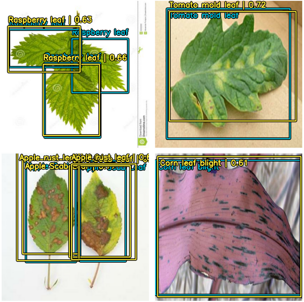
The metrics on our best model are:
- Loss: 0.4185
- mAP: 0.2182
- Validation Loss: 0.4584
- Validation mAP: 0.2916
Respectable, but this can be improved. More on this in the conclusion. (Note: I noticed that MultiClassNonMaxSuppression does not seem to be working correctly. The bottom left image shown above clearly has boxes that overlap with more than 20% of their area, yet the lower confidence box is not suppressed. This is something I will have to look more into.)
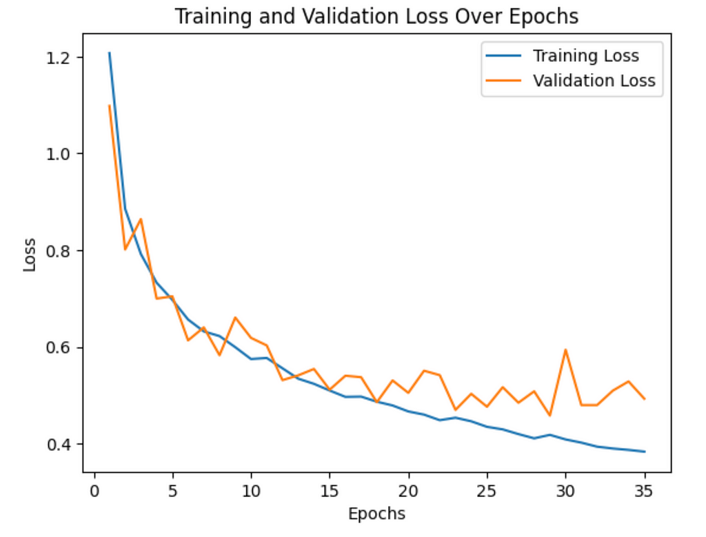
Here is a plot of our training and validation losses per epoch. Some overfitting is seen. Also, it may be wise to add in a learning rate schedule to decrease the learning rate over time. This may help resolve the issue of large jumps being made near the end of training.
Conclusion
If you have made it this far give yourself a pat on the back! Object detection is among the more difficult tasks in computer vision. Luckily for us we have the new KerasCV library to make our lives easier. To summarize the workflow for creating an object detection pipeline:
- Begin by visualizing your dataset. Ask yourself questions like: “What is my bounding box format? Is it xyxy? Relxyxy? How many classes am I dealing with?” Make sure to create a function similar to visualize_dataset to look at your images and bounding boxes.
- Convert whatever format of data you have into the “dictionary within a dictionary” format that KerasCV wants. Using a TensorFlow Dataset object to hold the data is especially helpful.
- Do some basic pre-processing, such as image re-sizing and data augmentation. KerasCV makes this fairly simple. Take care to read the literature on your model of choice to make sure the image sizes are appropriate.
- Convert the dictionaries back into tuples for training.
- Select an optimizer (Adam is an easy choice), two loss functions (focal for the class loss and L1 smooth for the box loss are easy choices), and metrics (COCO metrics are an easy choice).
- Visualizing your detections during training can be instructive to see what sorts of objects your model is missing.
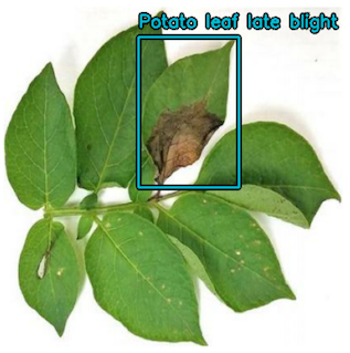
One of the primary next steps would be to clean up the dataset. For example, take a look at the image above. The labelers correctly identified the potato leaf late blight, but what about all of the other healthy potato leaves? Why were these not labeled as potato leaf? Looking at the health check tab on the Roboflow website, you can see that some classes are vastly underrepresented in the dataset:

[2] A. Géron, , DeepLearning.AI
[4] D. Singh, N. Jain, P. Jain, P. Kayal, S. Kumawat, N. Batra, (2017), CVPR 2017
[6] T. Lin, P. Goyal, R. Girshick, K. He, P. Dollar, was originally published in Towards Data Science on Medium, where people are continuing the conversation by highlighting and responding to this story.

SOCIAL SHARE CARD GENERATOR