A walk-through of cost computation, gradient descent, and regularization using Boston Housing dataset
Linear Regression seems old and naive when Large Language Models (LLMs) dominate people’s attention through their sophistication recently. Is there still a point of understanding it?
My answer is “Yes”, because it’s a building block of more complex models, including LLMs.
Creating a Linear Regression model can be as easy as running 3 lines of code:
from sklearn.linear_model import LinearRegression
regressor = LinearRegression()
regressor.fit(X_train, y_train)
However, this doesn’t show us the structure of the model. To produce optimal modeling results, we need to understand what goes on behind the scenes. In this article, I’ll break down the process of implementing Linear Regression in Python using a simple dataset known as “Boston Housing”, step by step.
What is Linear Regression
Linear — when plotted in a 2-dimensional space, if the dots showing the relationship of predictor x and predicted variable y scatter along a straight line, then we think this relationship can be represented by this line.
Regression — a statistical method for estimating the relationship between one or more predictors (independent variables) and a predicted (dependent variable).
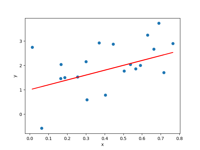
Linear Regression describes the predicted variable as a linear combination of the predictors. The line that abstracts this relationship is called line of best fit, see the red straight line in the below figure as an example.
Data Description
To keep our goal focused on illustrating the Linear Regression steps in Python, I picked the Boston Housing dataset, which is:
- Small — makes debugging easy
- Simple — so we spend less time in understanding the data or feature engineering
- Clean — requires minimum data cleaning
The dataset was first curated in .
Load data into Python using pandas:
import pandas as pd

# Load data
data = pd.read_excel("Boston_Housing.xlsx")
See the dataset’s number of rows (observations) and columns (variables):
data.shape
# (506, 14)
The modeling problem of our exercise is: given the attributes of a location, try to predict the median housing price of this location.
We store the target variable and predictors using 2 separate objects, x and y, following math and ML notations.
# Split up predictors and target
y = data['MEDV']
X = data.drop(columns=['MEDV'])
Visualize the dataset by histogram and scatter plot:
import numpy as np
import matplotlib.pyplot as plt

# Distribution of predictors and relationship with target
for col in X.columns:
    fig, ax = plt.subplots(1, 2, figsize=(6,2))
    ax[0].hist(X[col])
    ax[1].scatter(X[col], y)
    fig.suptitle(col)
    plt.show()
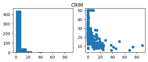
The point of visualizing the variables is to see if any transformation is needed for the variables, and identify the type of relationship between individual variables and target. For example, the target may have a linear relationship with some predictors, but polynomial relationship with others. This further infers which models to use for solving the problem.
Cost Computation
How well the model captures the relationship between the predictors and the target can be measured by how much the predicted results deviate from the ground truth. The function that quantifies this deviation is called Cost Function.
The smaller the cost is, the better the model captures the relationship the predictors and the target. This means, mathematically, the model training process aims to minimize the result of cost function.
There are different cost functions that can be used for regression problems: Sum of Squared Errors (SSE), Mean Squared Error (MSE), Mean Absolute Error (MAE)…
MSE is the most popular cost function used for Linear Regression, and is the default cost function in many statistical packages in R and Python. Here’s its math expression:

Note: The 2 in the denominator is there to make calculation neater.
To use MSE as our cost function, we can create the following function in Python:
def compute_cost(X, y, w, b):
    m = X.shape[0]

    f_wb = np.dot(X, w) + b
    cost = np.sum(np.power(f_wb - y, 2))

    total_cost = 1 / (2 * m) * cost

    return total_cost
Gradient Descent
Gradient — the slope of the tangent line at a certain point of the function. In multivariable calculus, gradient is a vector that points in the direction of the steepest ascent at a certain point.
Descent — moving towards the minimum of the cost function.
Gradient Descent — a method that iteratively adjusts the parameters in small steps, guided by the gradient, to reach the lowest point of a function. It is a way to numerically reach the desired parameters for Linear Regression.
In contrast, there’s a way to analytically solve for the optimal parameters — Ordinary Least Squares (OLS). See )
After scaling all the features to the same ranges, we can observe a smoother and more straight-forward path to global minimum of the cost function.
There are multiple ways to conduct feature scaling, and here we choose Standardization to turn all the features to have mean of 0 and standard deviation of 1.
Here’s how to standardize features in Python:
from sklearn.preprocessing import StandardScaler

standard_scaler = StandardScaler()
X_train_norm = standard_scaler.fit_transform(X_train)
X_test_norm = standard_scaler.transform(X_test)
Now we conduct Gradient Descent on the standardized dataset:
iterations = 1000
alpha = 1.0e-2

w_out, b_out, J_hist = gradient_descent(X_train_norm, y_train, w_init, b_init, compute_cost, compute_gradient, alpha, iterations)

print(f"Training result: w = {w_out}, b = {b_out}")
print(f"Training MSE = {J_hist[-1]}")
Training result: w = [-0.87200786  0.83235112 -0.35656148  0.70462672 -1.44874782  2.69272839
 -0.12111304 -2.55104665  0.89855827 -0.93374049 -2.151963   -3.7142413 ], b = 22.61090500500162
Training MSE = 9.95513733581214
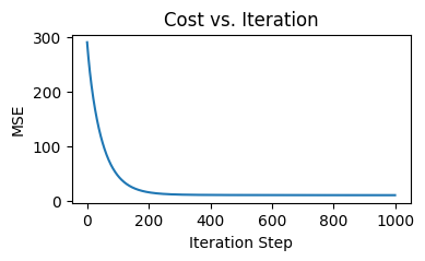
We get a steeper and smoother decline of cost before 200 iterations, compared to the previous round of training:
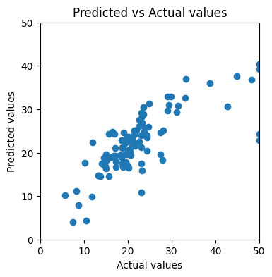
If we plot the predicted versus actual values again, we see the dots look much closer to a straight line:
To quantify the model performance on the test set:
mse = compute_mse(y_test, y_pred)
print(f"Test MSE = {mse}")
Test MSE = 35.66317674147827
We see an improvement from MSE of 132.84 to 35.66! Can we do more to improve the model?
Regularization — Ridge Regression
We notice that in the last round of training, the training MSE is 9.96, and the testing MSE is 35.66. Can we push the test set performance to be closer to training set?
Here comes Regularization. It penalizes large parameters to prevent the model from being too specific to the training set.
There are mainly 2 popular ways of regularization:
- L1 Regularization — uses the L1 norm (absolute values, a.k.a. “Manhattan norm”) of the weights as the penalty term.
- L2 Regularization — uses the L2 norm (squared values, a.k.a. “Euclidean norm”) of the weights as the penalty term.
Let’s first try Ridge Regression which uses L2 regularization as our new version of model. Its Gradient Descent process is easier to understand than LASSO Regression, which uses L1 regularization.
The cost function with L1 regularization looks like this:

Lambda controls the degree of penalty. When lambda is high, the level of penalty is high, then the model leans to underfitting.
We can turn the calculation into the following function:
def compute_cost_ridge(X, y, w, b, lambda_ = 1):
    m = X.shape[0]

    f_wb = np.dot(X, w) + b
    cost = np.sum(np.power(f_wb - y, 2))

    reg_cost = np.sum(np.power(w, 2))

    total_cost = 1 / (2 * m) * cost + (lambda_ / (2 * m)) * reg_cost

    return total_cost
For the Gradient Descent process, we use the following function to compute the gradients with regularization:
def compute_gradient_ridge(X, y, w, b, lambda_):
    m = X.shape[0]

    err = np.dot(X, w) + b - y
    dj_dw = np.dot(X.T, err) / m + (lambda_ / m) * w
    dj_db = np.sum(err) / m

    return dj_db, dj_dw
Combine the two steps together, we get the following Gradient Descent function for Ridge Regression:
def gradient_descent(X, y, w_in, b_in, cost_function, gradient_function, alpha, lambda_=0.7, num_iters=1000):
    J_history = []
    w = copy.deepcopy(w_in)
    b = b_in

    for i in range(num_iters):
        dj_db, dj_dw = gradient_function(X, y, w, b, lambda_)

        w = w - alpha * dj_dw
        b = b - alpha * dj_db

        cost = cost_function(X, y, w, b, lambda_)
        J_history.append(cost)

        if i % math.ceil(num_iters/10) == 0:
            print(f"Iteration {i:4d}: Cost {J_history[-1]:8.2f}")

    return w, b, J_history
Train the model on our standardized dataset:
iterations = 1000
alpha = 1.0e-2
lambda_ = 1

w_out, b_out, J_hist = gradient_descent(X_train_norm, y_train, w_init, b_init, compute_cost_ridge, compute_gradient_ridge, alpha, lambda_, iterations)
print(f"Training result: w = {w_out}, b = {b_out}")
print(f"Training MSE = {J_hist[-1]}")
Training result: w = [-0.86996629 0.82769399 -0.35944104 0.7051097 -1.43568137 2.69434668
-0.12306667 -2.53197524 0.88587909 -0.92817437 -2.14746836 -3.70146378], b = 22.61090500500162
Training MSE = 10.005991756561285
The training cost is slightly higher than our previous version of model.
The learning curve looks very similar to the one from the previous round:
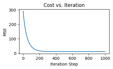
The predicted vs actual values plot looks almost identical to what we got from the previous round:
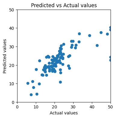
We got test set MSE of 35.69, which is slightly higher than the one without regularization.
Regularization — LASSO Regression
Finally, let’s try out LASSO Regression! LASSO stands for Least Absolute Shrinkage and Selection Operator.
This is the cost function with L2 regularization:

What’s tricky about the training process of LASSO Regression, is that the derivative of the absolute function is undefined at w=0. Therefore, Coordinate Descent is used in practice for LASSO Regression. It focuses on one coordinate at a time to find the minimum, and then switch to the next coordinate.
Here’s how we implement it in Python, inspired by .
First, we define the soft threshold function, which is the solution to the single variable optimization problem:
def soft_threshold(rho, lamda_):
    if rho < - lamda_:
        return (rho + lamda_)
    elif rho >  lamda_:
        return (rho - lamda_)
    else:
        return 0
Second, calculate the residuals of the prediction:
def compute_residuals(X, y, w, b):
    return y - (np.dot(X, w) + b)
Use the residual to calculate rho, which is the subderivative:
def compute_rho_j(X, y, w, b, j):
    X_k = np.delete(X, j, axis=1)    # remove the jth element
    w_k = np.delete(w, j)    # remove the jth element

    err = compute_residuals(X_k, y, w_k, b)

    X_j = X[:,j]
    rho_j = np.dot(X_j, err)

    return rho_j
Put everything together:
def coordinate_descent_lasso(X, y, w_in, b_in, cost_function, lambda_, num_iters=1000, tolerance=1e-4):
    J_history = []
    w = copy.deepcopy(w_in)
    b = b_in
    n = X.shape[1]

    for i in range(num_iters):
        # Update weights
        for j in range(n):
            X_j = X[:,j]
            rho_j = compute_rho_j(X, y, w, b, j)
            w[j] = soft_threshold(rho_j, lambda_) / np.sum(X_j ** 2)

        # Update bias
        b = np.mean(y - np.dot(X, w))
        err = compute_residuals(X, y, w, b)

        # Calculate total cost
        cost = cost_function(X, y, w, b, lambda_)
        J_history.append(cost)

        if i % math.ceil(num_iters/10) == 0:
            print(f"Iteration {i:4d}: Cost {J_history[-1]:8.2f}")

        # Check convergence
        if np.max(np.abs(err)) < tolerance:
            break

    return w, b, J_history
Apply it to our training set:
iterations = 1000
lambda_ = 1e-4
tolerance = 1e-4

w_out, b_out, J_hist = coordinate_descent_lasso(X_train_norm, y_train, w_init, b_init, compute_cost_lasso, lambda_, iterations, tolerance)
The training process converged drastically, compared to Gradient Descent on Ridge Regression:
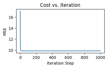
However, the training result is not significantly improved:
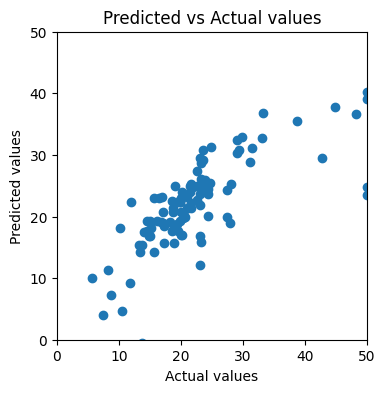
Eventually, we achieved MSE of 34.40, which is the lowest among the methods we tried.
Interpreting the Results
How do we interpret the model training results using human language? Let’s use the result of LASSO Regression as an example, since it has the best performance among the model variations we tried out.
We can get the weights and the bias by printing the w_out and b_out we got in the previous section:
print(f"Training result: w = {w_out}, b = {b_out}")Training result: w = [-0.86643384 0.82700157 -0.35437324 0.70320366 -1.44112303 2.69451013
-0.11649385 -2.53543865 0.88170899 -0.92308699 -2.15014264 -3.71479811], b = 22.61090500500162
In our case, there are 13 predictors, so this dataset has 13 dimensions. In each dimension, we can plot the predictor x_i against the target y as a scatterplot. The regression line’s slope is the weight w_i.
In details, the first dimension is “CRIM — per capita crime rate by town”, and our w_1 is -0.8664. This means, each unit of increase in x_i, y is expected to decrease by -0.8664 unit.
Note that we have scaled our dataset before we run the training process, so now we need to reverse that process to get the intuitive relationship between the predictor “per capita crime rate by town” and our target variable “median value of owner-occupied homes in $1000’s, at a specific location”.
To reverse the scaling, we need to get the vector of scales:
print(standard_scaler.scale_)
[8.12786482e+00 2.36076347e+01 6.98435113e+00 2.53975353e-01
 1.15057872e-01 6.93831576e-01 2.80721481e+01 2.07800639e+00
 8.65042138e+00 1.70645434e+02 2.19210336e+00 7.28999160e+00]
Here we find the scale we used for our first predictor: 8.1278. We divide the weight of -0.8664 by scale or 8.1278 to get -0.1066.
This means: when all other factors remains the same, if the per capita crime rate increases by 1 percentage point, the medium housing price of that location drops by $1000 * (-0.1066) = $106.6 in value.
Summary
This article unveiled the details of implementing Linear Regression in Python, going beyond just calling high level scikit-learn functions.
- We looked into the target of regression — minimizing the cost function, and wrote the cost function in Python.
- We broke down Gradient Descent process step by step.
- We created plotting functions to visualize the training process and assessing the results.
- We discussed ways to improve model performance, and found out that LASSO Regression achieved the lowest test MSE for our problem.
- Lastly, we used one predictor as an example to illustrate how the training result should be interpreted.
References
[1] A. Ng, Supervised Machine Learning: Regression and Classification (2022),
[3] Linear Regression (Python Implementation) (2024),
[5] X. Sicotte, Lasso regression: implementation of coordinate descent (2018),
[7] Fairlearn, Revisiting the Boston Housing Dataset,
[9] A. Gupta, Regularization in Machine Learning (2023),
on Medium, where people are continuing the conversation by highlighting and responding to this story.

SOCIAL SHARE CARD GENERATOR