PySpark techniques and strategies to tackle common performance challenges: A practical walkthrough
using PySpark, including ingestion, extraction, and visualization. However, despite its capacity to handle large datasets, performance bottlenecks can still arise under various scenarios such as extreme data distribution and complex data transformation workflow.
This article will examine different common performance issues in data processing with PySpark on on as its core building blocks, with data typically kept in memory by default. Whether executing computations (like joins and aggregations) or storing data across the cluster, all operations contribute to memory usage in a unified region.

If we design improperly, the available memory may become insufficient. This causes excess partitions to spill onto the disk, which results in performance degradation.
Caching and persisting intermediate results or frequently accessed datasets are common practices. While both cache and persist serve the same purposes, they may differ in their storage levels. The resources should be used optimally to ensure efficient read and write operations.
For example, if transformed data will be reused repeatedly for computations and algorithms across different subsequent stages, it is advisable to cache that data.
Code example: Assume we want to investigate different subsets of transaction records using a digital wallet as the payment method.
- Inefficient — Without caching
from pyspark.sql.functions import col

@time_decorator
def without_cache(data):
  # 1st filtering
  df2 = data.where(col("paymentMthd") == "Digital wallet")
  count = df2.count()

  # 2nd filtering
  df3 = df2.where(col("totalAmt") > 2000)
  count = df3.count()

  return count

display(without_cache(df))
- Efficient — Caching on a critical dataset
from pyspark.sql.functions import col

@time_decorator
def after_cache(data):
  # 1st filtering with cache
  df2 = data.where(col("paymentMthd") == "Digital wallet").cache()
  count = df2.count()

  # 2nd filtering
  df3 = df2.where(col("totalAmt") > 2000)
  count = df3.count()

  return count

display(after_cache(df))
After caching, even if we want to filter the transformed dataset with different transaction amount thresholds or other data dimensions, the execution times will still be more manageable.
#2 Shuffle
When we perform operations like joining DataFrames or grouping by data fields, shuffling occurs. This is necessary to redistribute all records across the cluster and to ensure those with the same key are on the same node. This in turn facilitates simultaneous processing and combining of the results.
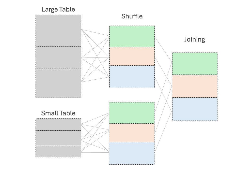
However, this shuffle operation is costly — high execution times and additional network overhead due to data movement between nodes.
To reduce shuffling, there are several strategies:
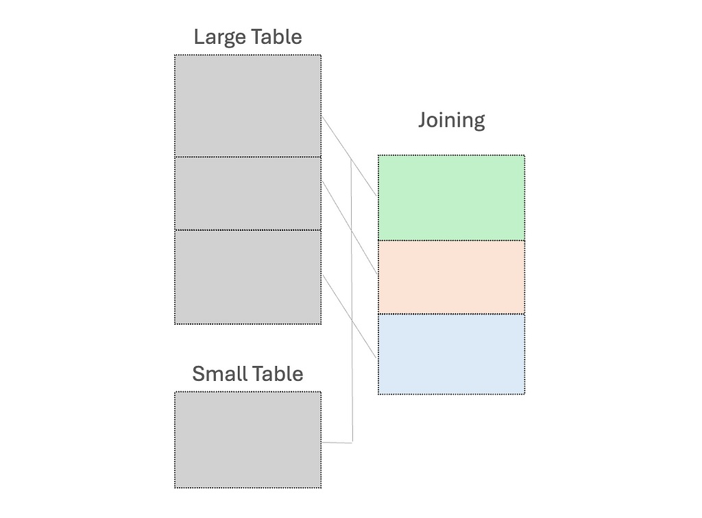
(1) Use broadcast variables for the small dataset, to send a read-only copy to every worker node for local processing
While “small” dataset is often defined by a maximum memory threshold of 8GB per executor, the ideal size for broadcasting should be determined through experimentation on specific case.
(2) Early filtering, to minimize the amount of data processed as early as possible; and
(3) Control the number of partitions to ensure optimal performance
Code examples: Assume we want to return the transaction records that match our list of states, along with their full names
- Inefficient — shuffle join between a large dataset and a small one
from pyspark.sql.functions import col

@time_decorator
def no_broadcast_var(data):
  # Create small dataframe
  small_data = [("CA", "California"), ("TX", "Texas"), ("FL", "Florida")]
  small_df = spark.createDataFrame(small_data, ["state", "stateLF"])

  # Perform joining
  result_no_broadcast = data.join(small_df, "state")

  return result_no_broadcast.count()

display(no_broadcast_var(df))
- Efficient — join the large dataset with the small one using a broadcast variable
from pyspark.sql.functions import col, broadcast

@time_decorator
def have_broadcast_var(data):
  small_data = [("CA", "California"), ("TX", "Texas"), ("FL", "Florida")]
  small_df = spark.createDataFrame(small_data, ["state", "stateFullName"])

  # Create broadcast variable and perform joining
  result_have_broadcast = data.join(broadcast(small_df), "state")

  return result_have_broadcast.count()

display(have_broadcast_var(df))
#3 Skewness
Data can sometimes be unevenly distributed, especially for data fields used as the key for processing. This leads to imbalanced partition sizes, in which some partitions are significantly larger or smaller than the average.
Since the execution performance is limited by the longest-running tasks, it is necessary to address the over-burdened nodes.
One common approach is salting. This works by adding randomized numbers to the skewed key so that there is a more uniform distribution across partitions. Let’s say when aggregating data based on the skewed key, we will aggregate using the salted key and then aggregate with the original key. Another method is re-partitioning, which increases the number of partitions to help distribute the data more evenly.
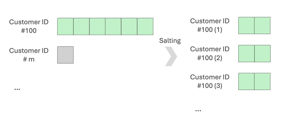
Code examples: We want to aggregate an asymmetric dataset, mainly skewed by customer ID #100.
- Inefficient — directly use the skewed key
from pyspark.sql.functions import col, desc

@time_decorator
def no_salting(data):
  # Perform aggregation
  agg_data = data.groupBy("customerID").agg({"totalAmt": "sum"}).sort(desc("sum(totalAmt)"))
  return agg_data

display(no_salting(df))
- Efficient — use the salting skewed key for aggregation
from pyspark.sql.functions import col, lit, concat, rand, split, desc

@time_decorator
def have_salting(data):
  # Salt the customerID by adding the suffix
  salted_data = data.withColumn("salt", (rand() * 8).cast("int")) \
                .withColumn("saltedCustomerID", concat(col("customerID"), lit("_"), col("salt")))

  # Perform aggregation
 agg_data = salted_data.groupBy("saltedCustomerID").agg({"totalAmt": "sum"})

 # Remove salt for further aggregation
 final_result = agg_data.withColumn("customerID", split(col("saltedCustomerID"), "_")[0]).groupBy("customerID").agg({"sum(totalAmt)": "sum"}).sort(desc("sum(sum(totalAmt))"))

 return final_result

display(have_salting(df))
A random prefix or suffix to the skewed keys will both work. Generally, 5 to 10 random values are a good starting point to balance between spreading out the data and maintaining high complexity.
#4 Serialization
People often prefer using , which can handle tasks such as aggregation, arrays/maps operations, date/time stamps, and JSON data processing. If the built-in functions do not satisfy your desired tasks indeed, we can consider using has been newly addressed for dynamic planning and re-planning of queries based on runtime stats. This supports different features of query re-optimization that occur during query execution, which creates a great optimization technique. However, understanding data characteristics during the initial design is still essential, as it informs better strategies for writing effective codes and queries while using AQE for fine-tuning.
Before you go
If you enjoy this reading, I invite you to follow my . By doing so, you can stay updated with exciting content related to data science side projects, Machine Learning Operations (MLOps) demonstrations, and project management methodologies.
on Medium, where people are continuing the conversation by highlighting and responding to this story.

SOCIAL SHARE CARD GENERATOR