Vision Transformer with BatchNorm: Optimizing the depth

Vision Transformer with BatchNorm

How integrating BatchNorm in a standard Vision transformer architecture leads to faster convergence and a more stable network

Introduction

The ViT-type models which integrate Batch Normalization (BatchNorm) in their architecture. BatchNorm is known to make a deep neural network converge faster — a network with BatchNorm achieves higher accuracy compared to the base-line model when trained over the same number of epochs. This in turn speeds up training. BatchNorm also acts as an efficient regularizer for the network, and allows a model to be trained with a higher learning rate. The main goal of this article is to investigate whether introducing BatchNorm can lead to similar effects in a Vision Transformer.

For the sake of concreteness, I will focus on a model where a BatchNorm layer is introduced in the Feedforward Network (FFN) within the transformer encoder of the ViT, and the LayerNorm preceding the FFN is omitted. Everywhere else in the transformer — including the self-attention module — one continues to use LayerNorm. I will refer to this version of ViT as ViTBNFFN — Vision Transformer with BatchNorm in the Feedforward Network. I will train and test this model on the MNIST dataset with image augmentations and compare the Top-1 accuracy of the model with that of the standard ViT over a number of epochs. I will choose identical architectural configuration for the two models (i.e. identical width, depth, patch size and so on) so that one can effectively isolate the effect of the BatchNorm layer.

Here’s a quick summary of the main findings:

1. For a reasonable choice of hyperparameters (learning rate and batch size), ViTBNFFN does converge faster than ViT, provided the transformer depth (i.e number of layers in the encoder) is sufficiently large.
2. As one increases the learning rate, ViTBNFFN turns out to be more stable than ViT, especially at larger depths.

I will open with a brief discussion on BatchNorm in a deep neural network, illustrating some of the properties mentioned above using a concrete example. I will then discuss in detail the architecture of the model ViTBNFFN. Finally, I will take a deep dive into the numerical experiments that study the effects of BatchNorm in the Vision Transformer.

The Dataset : MNIST with Image Augmentation

Let us begin by introducing the augmented MNIST dataset which I will use for all the numerical experiments described in this article. The training and test datasets are given by the function get_datasets_mnist() as shown in Code Block 1.

Batch Normalization in a Deep Neural Network

Let us give a quick review of how BatchNorm improves the performance of a deep neural network. Suppose zᵃᵢ denotes the input for a given layer of a deep neural network, where a is the batch index which runs from a=1,…, Nₛ and i is the feature index running from i=1,…, C. The BatchNorm operation then involves the following steps:

1. For a given feature index i, one first computes the mean and the variance over the batch of size Nₛ i.e.

2. One normalizes the input using the mean and variance computed above (with ϵ being a small positive number):

3. Finally, one shifts and rescales the normalized input for every feature i:

where there is no summation over the index i, and the parameters (γᵢ, βᵢ) are trainable.

Consider a deep neural network for classifying the MNIST dataset. I will choose a network consisting of 3 fully-connected hidden layers, with 100 activations each, where each hidden layer is endowed with a sigmoid activation function. The last hidden layer feeds into a classification layer with 10 activations corresponding to the 10 classes of the MNIST dataset. The input to this neural network is a 2d-tensor of shape b × 28² — where b is the batch size and each 28 × 28 MNIST image is reshaped into a 28²-dimensional vector. In this case, the feature index runs from i=1, …, 28².

This model is similar to the one discussed in the original BatchNorm for more details). This makes the network significantly more resistant to instabilities arising out of a high learning rate.

To demonstrate this explicitly for the models at hand, let us train them at a much higher learning rate lr=0.1 — the test accuracy and the training losses for the models in this case are given in Figure 2.

The high learning rate manifestly renders the DNN unstable. The model with BatchNorm, however, is perfectly well-behaved! A more instructive way to visualize this behavior is to plot the accuracy curves for the two learning rates in a single graph, as shown in Figure 3.

While the model DNN_d3 stops training at the high learning rate, the impact on the performance of DNNBN_d3 is significantly milder. BatchNorm therefore allows one to train a model at a higher learning rate, providing yet another way to speed up training.

The Model ViTBNFFN : BatchNorm in the FeedForward Network

Let us begin by briefly reviewing the architecture of the standard Vision Transformer for image classification tasks, as shown in the schematic diagram of Figure 4. For more details, I refer the reader to my previous

The built-in BatchNorm class in PyTorch always takes the first index of a tensor as the batch index and the second index as the feature index. Therefore, one needs to transform our 3d tensor with shape b × N × dₑ to a tensor of shape b × dₑ × N before applying BatchNorm, and transforming it back to b × N × dₑ afterwards. In addition, I have used the 2d BatchNorm class (since it is slightly faster than the 1d BatchNorm). This requires promoting the 3d tensor to a 4d tensor of shape b × dₑ × N × 1 (line 16) and transforming it back (line 18) to a 3d tensor of shape b × N × dₑ. One can use the 1d BatchNorm class without changing any of the results presented in the section.

The Experiment

With a fixed learning rate and batch size, I will train and test the two models — ViT and ViTBNFFN — on the augmented MNIST dataset for 10 epochs and compare the Top-1 accuracies on the validation dataset. Since we are interested in understanding the effects of BatchNorm, we will have to compare the two models with identical configurations. The experiment will be repeated at different depths of the transformer encoder keeping the rest of the model configuration unchanged. The specific configuration for the two models that I use in this experiment is given as follows :

1. Embedding layer: An MNIST image is a grey-scale image of size 28× 28. The patch size is p= 7, which implies that the number of tokens is 16 + 1 =17 including the CLS token. The embedding dimension is dₑ = 64.
2. Transformer encoder: The MHSA submodule has nₕ = 8 heads with head dimension dₕ=64. The hidden dimension of the FFN is d_mlp = 128. The depth of the encoder will be the only variable parameter in this architecture.
3. MLP head: The MLP head will simply consist of a linear layer.

The training and testing batch sizes will be fixed at 100 and 5000 respectively for all the epochs, with CrossEntropyLoss() as the loss function and Adam optimizer. The dropout parameters are set to zero in both the embedding layer as well as the encoder. I have used the NVIDIA L4 Tensor Core GPU available at Google Colab for all the runs, which have been recorded using the tracking feature of MLFlow.

Let us start by training and testing the models at the learning rate lr= 0.003. Figure 8 below summarizes the four graphs which plot the accuracy curves of the two models at depths d=4, 5, 6 and 7 respectively. In these graphs, the notation ViT_dn (ViTBNFFN_dn) denotes ViT (ViTBNFFN) with depth of the encoder d=n and the rest of the model configuration being the same as specified above.

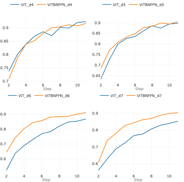
For d= 4 and d= 5 (the top row of graphs), the accuracies of the two models are comparable — for d=4 (top left) ViT does somewhat better, while for d=5 (top right) ViTBNFFN surpasses ViT marginally. For d < 4, the accuracies remain comparable. However, for d=6 and d=7 (the bottom row of graphs), ViTBNFFN does significantly better than ViT. One can check that this qualitative feature remains the same for any depth d ≥ 6.

Let us repeat the experiment at a slightly higher learning rate lr = 0.005. The accuracy curves of the two models at depths d=1, 2, 3 and 4 respectively are summarized in Figure 9.

For d= 1 and d= 2 (the top row of graphs), the accuracies of the two models are comparable — for d=1 ViT does somewhat better, while for d=2 they are almost indistinguishable. For d=3 (bottom left), ViTBNFFN achieves a slightly higher accuracy than ViT. For d=4 (bottom right), however, ViTBNFFN does significantly better than ViT and this qualitative feature remains the same for any depth d ≥ 4.

Therefore, for a reasonable choice of learning rate and batch size, ViTBNFFN converges significantly faster than ViT beyond a critical depth of the transformer encoder. For the range of hyperparameters I consider, it seems that this critical depth gets smaller with increasing learning rate at a fixed batch size.

For the deep neural network example, we saw that the impact of a high learning rate is significantly milder on the network with BatchNorm. Is there something analogous that happens for a Vision Transformer? This is addressed in Figure 10. Here each graph plots the accuracy curves of a given model at a given depth for two different learning rates lr=0.003 and lr=0.005. The first column of graphs corresponds to ViT for d=2, 3 and 4 (top to bottom) while the second column corresponds to ViTBNFFN for the same depths.

Consider d=2 — given by the top row of graphs — ViT and ViTBNFFN are comparably impacted as one increases the learning rate. For d = 3 — given by the second row of graphs — the difference is significant. ViT achieves a much lower accuracy at the higher learning rate — the accuracy drops from about 91% to around 78% at the end of epoch 10. On the other hand, for ViTBNFFN, the accuracy at the end of epoch 10 drops from about 92% to about 90%. This qualitative feature remains the same at higher depths too — see the bottom row of graphs which corresponds to d=4. Therefore, the impact of the higher learning rate on ViTBNFFN looks significantly milder for sufficiently large depth of the transformer encoder.

Conclusion

In this article, I have studied the effects of introducing a BatchNorm layer inside the FeedForward Network of the transformer encoder in a Vision Transformer. Comparing the models on an augmented MNIST dataset, there are two main lessons that one may draw. Firstly, for a transformer of sufficient depth and for a reasonable choice of hyperparameters, the model with BatchNorm achieves significantly higher accuracy compared to the standard ViT. This faster convergence can greatly speed up training. Secondly, similar to our intuition for deep neural networks, the Vision Transformer with BatchNorm is more resilient to a higher learning rate, if the encoder is sufficiently deep.

Thanks for reading! If you have made it to the end of the article and enjoyed it, please leave claps and/or comments and follow me for more content! Unless otherwise stated, all images and graphs used in this article were generated by the author.

on Medium, where people are continuing the conversation by highlighting and responding to this story.