Building a Vision Inspection CNN for an Industrial Application

A step-by-step approach using PyTorch

In this article, we develop and code a Convolutional Neural Network (CNN) for a vision inspection classification task in the automotive electronics industry. Along the way, we study the concept and math of convolutional layers in depth, and we examine what CNNs actually see and which parts of the image lead them to their decisions.

Table of Content

Part 1: Conceptual background
Part 2: Defining and coding the CNN
Part 3: Using the trained model in production
Part 4: What did the CNN consider in its “decision”?

Part 1: Conceptual background

1.1 The task: Classify an industrial component as good or scrap

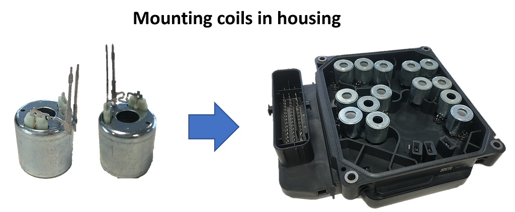
In one station of an automatic assembly line, coils with two protruding metal pins have to be positioned precisely in a housing. The metal pins are inserted into small plug sockets. In some cases, the pins are slightly bent and therefore cannot be joined by a machine. It is the task of the visual inspection to identify these coils, so that they can be sorted out automatically.

For the inspection, each coil is picked up individually and held in front of a screen. In this position, a camera takes a grayscale image. This is then examined by the CNN and classified as good or scrap.

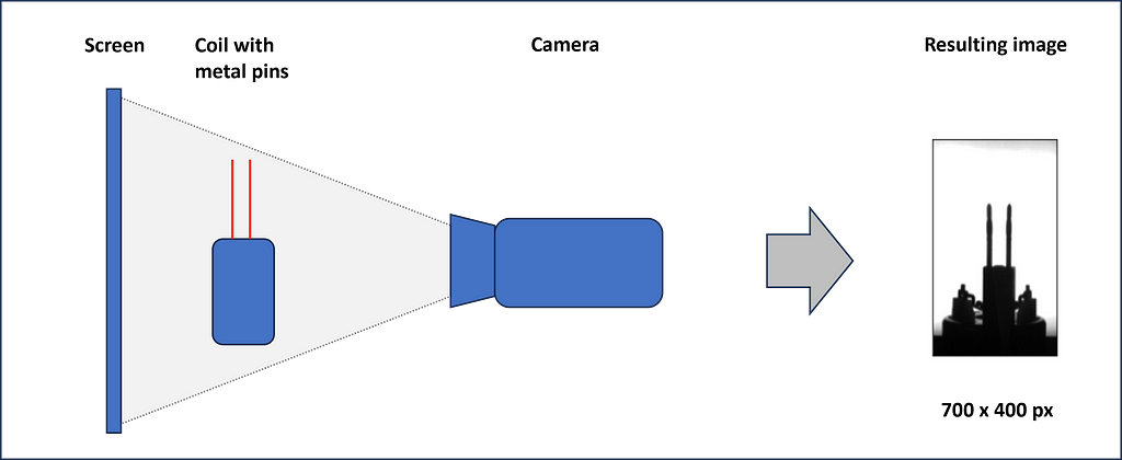
Now, we want to define a convolutional neural network that is able to process the images and learn from pre-classified labels.

1.2 What is a Convolutional Neural Network (CNN)?

Convolutional Neural Networks are a combination of convolutional filters followed by a fully connected Neural Network (NN). CNNs are often used for image processing, like face recognition or visual inspection tasks, like in our case. Convolutional filters are matrix operations that slide over the images and recalculate each pixel of the image. We will study convolutional filters later in the article. The weights of the filters are not preset (as, e.g. the sharpen function in Photoshop) but instead are learned from the data during training.

1.3 Architecture of a Convolutional Neural Network

Let’s check an example of the architecture of a CNN. For our convenience, we choose the model we will implement later.

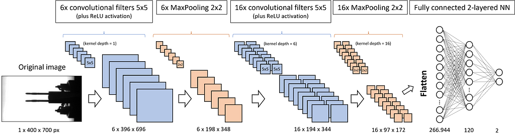
We want to feed the CNN with our inspection images of size 400 px in height and 700 px in width. Since the images are grayscale, the corresponding PyTorch tensor is of size 1x400x700. If we used a colored image, we would have 3 incoming channels: one for red, one for green and one for blue (RGB). In this case the tensor would be 3x400x700.

The first convolutional filter has 6 kernels of size 5x5 that slide over the image and produce 6 independent new images, called feature maps, of slightly reduced size (6x396x696). The ReLU activation is not explicitly shown in Fig. 3. It does not change the dimensions of the tensors but sets all negative values to zero. ReLU is followed by the MaxPooling layer with a kernel size of 2x2. It halves the width and height of each image.

All three layers — convolution, ReLU, and MaxPooling — are implemented a second time. This finally brings us 16 feature maps with images of height 97 pixels and width 172 pixels. Next, all the matrix values are flattened and fed into the equally sized first layer of a fully connected neural network. Its second layer is already reduced to 120 neurons. The third and output layer has only 2 neurons: one represents the label “OK”, and the other the label “not OK” or “scrap”.

If you are not yet clear about the changes in the dimensions, please be patient. We study how the different kinds of layers — convolution, ReLU, and MaxPooling — work in detail and impact the tensor dimensions in the next chapters.

1.4 Convolutional filter layers

Convolutional filters have the task of finding typical structures/patterns in an image. Frequently used kernel sizes are 3x3 or 5x5. The 9, respectively 25, weights of the kernel are not specified upfront but learned during training (here we assume that we have only one input channel; otherwise, the number of weights multiply by input channels). The kernels slide over the matrix representation of the image (each input channel has its own kernel) with a defined stride in the horizontal and vertical directions. The corresponding values of the kernel and the matrix are multiplied and summed up. The summation results of each sliding position form the new image, which we call the feature map. We can specify multiple kernels in a convolutional layer. In this case, we receive multiple feature maps as the result. The kernel slides over the matrix from left to right and top to bottom. Therefore, Fig. 4 shows the kernel in its fifth sliding position (not counting the “…”). We see three input channels for the colors red, green, and blue (RGB). Each channel has one kernel only. In real applications, we often define multiple kernels per input channel.

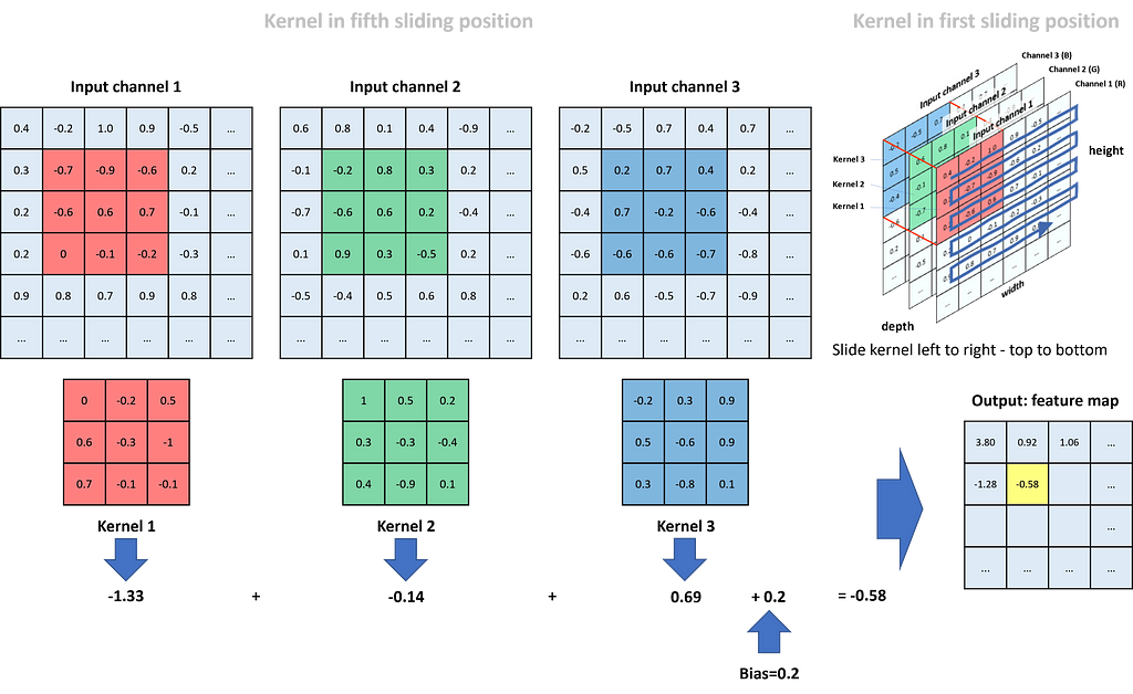
Kernel 1 does its work for the red input channel. In the shown position, we compute the respective new value in the feature map as (-0.7)*0 + (-0.9)*(-0.2) + (-0.6)*0.5 + (-0.6)*0.6 + 0.6*(-0.3) + 0.7*(-1) + 0*0.7 + (-0.1)*(-0.1) + (-0.2)*(-0.1) = (-1.33). The respective calculation for the green channel (kernel 2) adds up to -0.14, and for the blue channel (kernel 3) to 0.69. To receive the final value in the feature map for this specific sliding position, we sum up all three channel values and add a bias (bias and all kernel weights are defined during training of the CNN): (-1.33) + (-0.14) + 0.69 + 0.2 = -0.58. The value is placed in the position of the feature map highlighted in yellow.

Finally, if we compare the size of the input matrices to the size of the feature map, we see that through the kernel operations, we lost two rows in height and two columns in width.

1.5 ReLU activation layers

After the convolution, the feature maps are passed through the activation layer. Activation is required to give the network nonlinear capabilities. The two most frequently used activation methods are Sigmoid and ReLU (Rectified Linear Unit). ReLU activation sets all negative values to zero while leaving positive values unchanged.

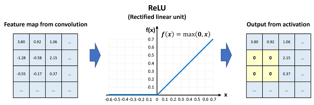
In Fig. 5, we see that the values of the feature map pass the ReLU activation element-wise.

ReLU activation has no impact on the dimensions of the feature map.

1.6 MaxPooling layers

Pooling layers have mainly the task of reducing the size of the feature maps while keeping the important information for the classification. In general, we can pool by calculating the average of an area in the kernel or returning the maximum. MaxPooling is more beneficial in most applications because it reduces the noise in the data. Typical kernel sizes for pooling are 2x2 or 3x3.

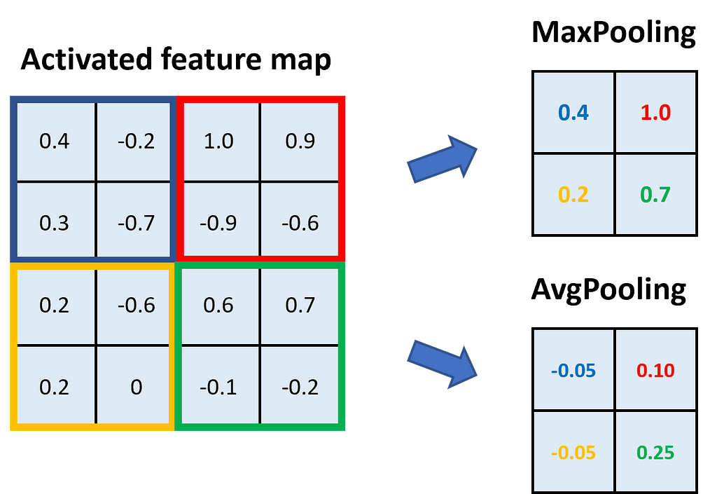
In Fig. 6, we see an example of MaxPooling and AvgPooling with a kernel size of 2x2. The feature map is divided into areas of the kernel size, and within those areas, we take either the maximum (→ MaxPooling) or the average (→ AvgPooling).

Through pooling with a kernel size of 2x2, we halve the height and width of the feature map.

1.7 Tensor dimensions in the Convolutional Neural Network

Now that we have studied the convolutional filters, the ReLU activation, and the pooling, we can revise Fig. 3 and the dimensions of the tensors. We start with an image of size 400x700. Since it is grayscale, it has only 1 channel, and the corresponding tensor is of size 1x400x700. We apply 6 convolutional filters of size 5x5 with a stride of 1x1 to the image. Each filter returns its own feature map, so we receive 6 of them. Due to the larger kernel compared to Fig. 4 (5x5 instead of 3x3), this time we lose 4 columns and 4 rows in the convolution. This means the returning tensor has the size 6x396x696.

In the next step, we apply MaxPooling with a 2x2 kernel to the feature maps (each map has its own pooling kernel). As we have learned, this reduces the maps’ dimensions by a factor of 2. Accordingly, the tensor is now of size 6x198x348.

Now we apply 16 convolutional filters of size 5x5. Each of them has a kernel depth of 6, which means that each filter provides a separate layer for the 6 channels of the input tensor. Each kernel layer slides over one of the 6 input channels, as studied in Fig. 4, and the 6 returning feature maps are added up to one. So far, we considered only one convolutional filter, but we have 16 of them. That is why we receive 16 new feature maps, each 4 columns and 4 rows smaller than the input. The tensor size is now 16x194x344.

Once more, we apply MaxPooling with a kernel size of 2x2. Since this halves the feature maps, we now have a tensor size of 16x97x172.
Finally, the tensor is flattened, which means we line up all of the 16*97*172 = 266,944 values and feed them into a fully connected neural network of corresponding size.

Part 2: Defining and coding the CNN

Conceptually, we have everything we need. Now, let’s go into the industrial use case as described in chapter 1.1.

2.1 Load the required libraries

We are going to use a couple of PyTorch libraries for data loading, sampling, and the model itself. Additionally, we load matplotlib.pyplot for visualization and PIL for transforming the images.

import torch
import torch.nn as nn
from torch.utils.data import DataLoader, Dataset
from torch.utils.data.sampler import WeightedRandomSampler
from torch.utils.data import random_split
from torchvision import datasets, transforms
import matplotlib.pyplot as plt
import numpy as np
from PIL import Image
import os
import warnings
warnings.filterwarnings("ignore")

2.2 Configure your device and specify hyperparameters

In device, we store ‘cuda’ or ‘cpu’, depending on whether or not your computer has a GPU available. minibatch_size defines how many images will be processed in one matrix operation during the training of the model. learning_rate specifies the magnitude of parameter adjustment during backpropagation, and epochs defines how often we process the whole set of training data in the training phase.

# Device configuration
device = torch.device('cuda' if torch.cuda.is_available() else 'cpu')
print(f"Using {device} device")

# Specify hyperparameters
minibatch_size = 10
learning_rate = 0.01
epochs = 60

2.3 Custom loader function

For loading the images, we define a custom_loader. It opens the images in binary mode, crops the inner 700x400 pixels of the image, loads them into memory, and returns the loaded images. As the path to the images, we define the relative path data/Coil_Vision/01_train_val_test. Please make sure that the data is stored in your working directory. You can download the files from my Dropbox as was originally published in Towards Data Science on Medium, where people are continuing the conversation by highlighting and responding to this story.