How to Interpret Matrix Expressions — Transformations

Matrix algebra for a data scientist

This article begins a series for anyone who finds matrix algebra overwhelming. My goal is to turn what you’re afraid of into what you’re fascinated by. You’ll find it especially helpful if you want to understand machine learning concepts and methods.

Table of contents:

1. Introduction
2. Prerequisites
3. Matrix-vector multiplication
4. Transposition
5. Composition of transformations
6. Inverse transformation
7. Non-invertible transformations
8. Determinant
9. Non-square matrices
10. Inverse and Transpose: similarities and differences
11. Translation by a vector
12. Final words

1. Introduction

You’ve probably noticed that while it’s easy to find materials explaining matrix computation algorithms, it’s harder to find ones that teach how to interpret complex matrix expressions. I’m addressing this gap with my series, focused on the part of matrix algebra that is most commonly used by data scientists.

We’ll focus more on concrete examples rather than general formulas. I’d rather sacrifice generality for the sake of clarity and readability. I’ll often appeal to your imagination and intuition, hoping my materials will inspire you to explore more formal resources on these topics. For precise definitions and general formulas, I’d recommend you look at some good textbooks: the classic one on linear algebra¹ and the other focused on machine learning².

This part will teach you

to see a matrix as a representation of the transformation applied to data.

Let’s get started then — let me take the lead through the world of matrices.

2. Prerequisites

I’m guessing you can handle the expressions that follow.

This is the dot product written using a row vector and a column vector:

A matrix is a rectangular array of symbols arranged in rows and columns. Here is an example of a matrix with two rows and three columns:

You can view it as a sequence of columns

or a sequence of rows stacked one on top of another:

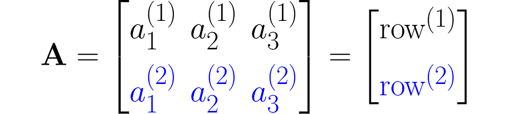
As you can see, I used superscripts for rows and subscripts for columns. In machine learning, it’s important to clearly distinguish between observations, represented as vectors, and features, which are arranged in rows.

Other interesting ways to represent this matrix are A₂ₓ₃ and A[aᵢ⁽ʲ ⁾].

Multiplying two matrices A and B results in a third matrix C = AB containing the scalar products of each row of A with each column of B, arranged accordingly. Below is an example for C₂ₓ₂ = A₂ₓ₃B₃ₓ₂.

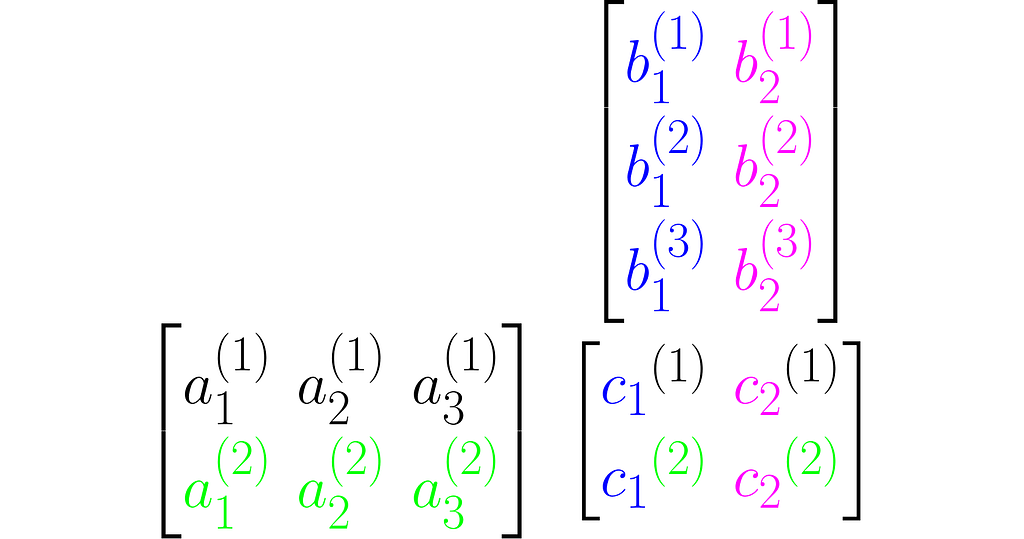
where cᵢ⁽ʲ ⁾ is the scalar product of the i-th column of the matrix B and the j-th row of matrix A:

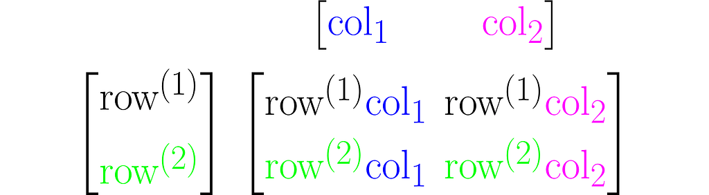
Note that this definition of multiplication requires the number of rows of the left matrix to match the number of columns of the right matrix. In other words, the inner dimensions of the matrices must match.

Make sure you can manually multiply matrices with arbitrary entries. You can use the following code to check the result or to practice multiplying matrices.

import numpy as np

# Matrices to be multiplied
A = [
    [ 1, 0, 2],
    [-2, 1, 1]
]

B = [
    [ 0, 3, 1],
    [-3, 1, 1],
    [-2, 2, 1]
]

# Convert to numpy array
A = np.array(A)
B = np.array(B)

# Multiply A by B (if possible)
try:
    C = A @ B
    print(f'A B = \n{C}\n')
except:
    print("""ValueError:
The number of rows in matrix A does not match 
the number of columns in matrix B
""")

#  and in the reverse order, B by A (if possible)
try:
    D = B @ A
    print(f'B A =\n{D}')
except:
    print("""ValueError:
The number of rows in matrix B does not match 
the number of columns in matrix A
""")

A B = 
[[-4  7]
 [-5 -3]]

B A =
[[-6  3  3]
 [-5  1 -5]
 [-6  2 -2]]

3. Matrix-vector multiplication

In this section, I will explain the effect of matrix multiplication on vectors. The vector x is multiplied by the matrix A, producing a new vector y:

This is a common operation in data science, as it enables a linear transformation of data. The use of matrices to represent linear transformations is highly advantageous, as you will soon see in the following examples.

Below, you can see your grid space and your standard basis vectors: blue for the x⁽¹⁾ direction and magenta for the x⁽²⁾ direction.

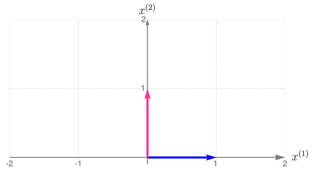
A good starting point is to work with transformations that map two-dimensional vectors x into two-dimensional vectors y in the same grid space.

Describing the desired transformation is a simple trick. You just need to say how the coordinates of the basis vectors change after the transformation and use these new coordinates as the columns of the matrix A.

As an example, consider a linear transformation that produces the effect illustrated below. The standard basis vectors are drawn lightly, while the transformed vectors are shown more clearly.

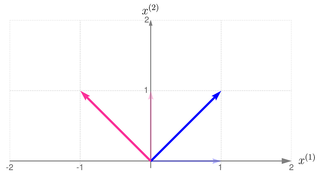
From the comparison of the basis vectors before and after the transformation, you can observe that the transformation involves a 45-degree counterclockwise rotation about the origin, along with an elongation of the vectors.

This effect can be achieved using the matrix A, composed as follows:

The first column of the matrix contains the coordinates of the first basis vector after the transformation, and the second column contains those of the second basis vector.

The equation (1) then takes the form

Let’s take two example points x₁and x₂ :

and transform them into the vectors y₁​ and y₂ :

I encourage you to do these calculations by hand first, and then switch to using a program like this:

import numpy as np

# Transformation matrix
A = np.array([
    [1, -1],
    [1,  1]
])

# Points (vectors) to be transformed using matrix A
points = [
    np.array([1, 1/2]),
    np.array([-1/4, 5/4])
]

# Print out the transformed points (vectors)
for i, x in enumerate(points):
    y = A @ x
    print(f'y_{i} = {y}')

y_0 = [0.5 1.5]
y_1 = [-1.5  1. ]

The plot below shows the results.

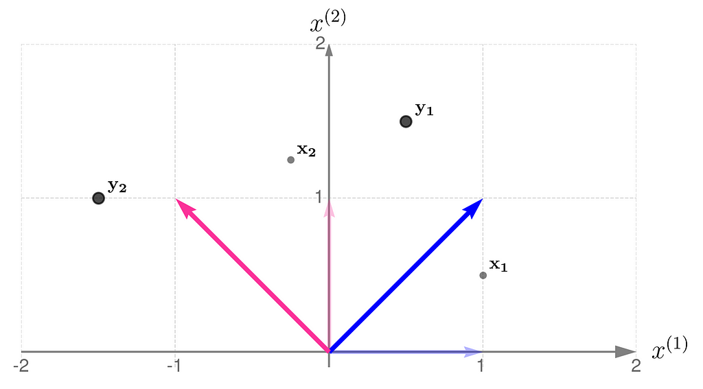
The x points are gray and smaller, while their transformed counterparts y have black edges and are bigger. If you’d prefer to think of these points as arrowheads, here’s the corresponding illustration:

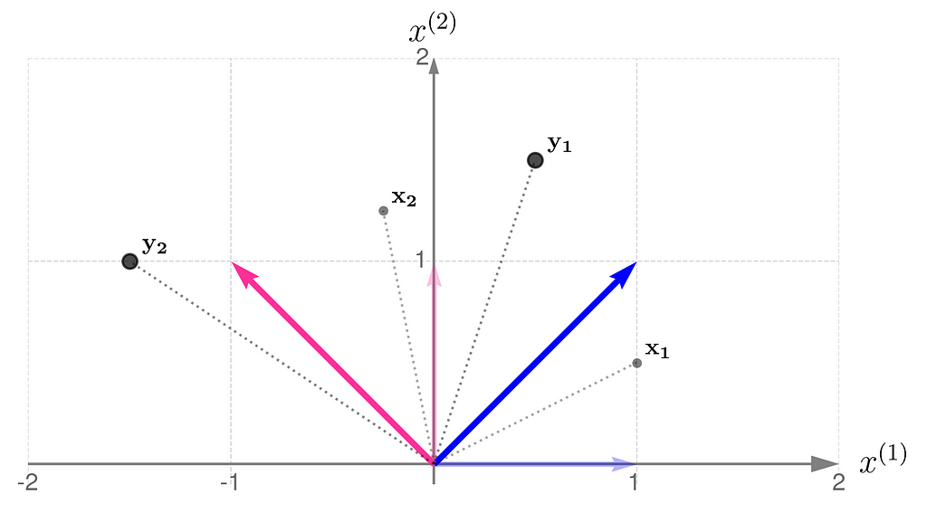
Now you can see more clearly that the points have been rotated around the origin and pushed a little away.

Let’s examine another matrix:

and see how the transformation

affects the points on the grid lines:

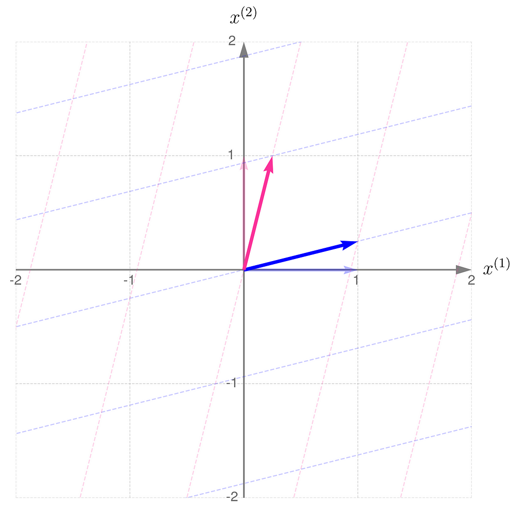
Compare the result with that obtained using B/2, which corresponds to dividing all elements of the matrix B by 2:

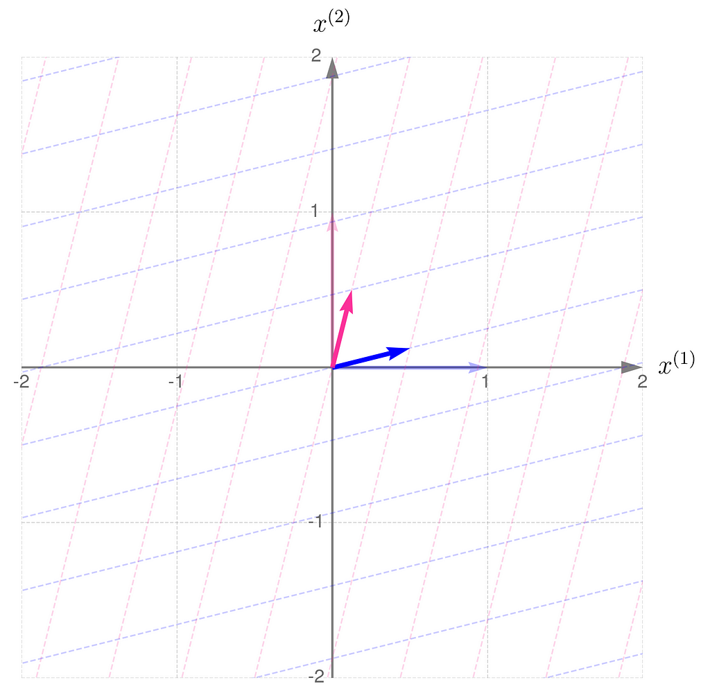
In general, a linear transformation:

• ensures that straight lines remain straight,
• keeps parallel lines parallel,
• scales the distances between them by a uniform factor.

To keep things concise, I’ll use ‘transformation A‘ throughout the text instead of the full phrase ‘transformation represented by matrix A’.

Let’s return to the matrix

and apply the transformation to a few sample points.

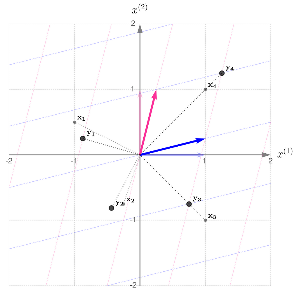
Notice the following:

• point x₁​ has been rotated counterclockwise and brought closer to the origin,
• point x₂​, on the other hand, has been rotated clockwise and pushed away from the origin,
• point x₃​ has only been scaled down, meaning it’s moved closer to the origin while keeping its direction,
• point x₄ has undergone a similar transformation, but has been scaled up.

The transformation compresses in the x⁽¹⁾-direction and stretches in the x⁽²⁾-direction. You can think of the grid lines as behaving like an accordion.

Directions such as those represented by the vectors x₃ and x₄ play an important role in machine learning, but that’s a story for another time.

For now, we can call them eigen-directions, because vectors along these directions might only be scaled by the transformation, without being rotated. Every transformation, except for rotations, has its own set of eigen-directions.

4. Transposition

Recall that the transformation matrix is constructed by stacking the transformed basis vectors in columns. Perhaps you’d like to see what happens if we swap the rows and columns afterwards (the transposition).

Let us take, for example, the matrix

where Aᵀ stands for the transposed matrix.

From a geometric perspective, the coordinates of the first new basis vector come from the first coordinates of all the old basis vectors, the second from the second coordinates, and so on.

In NumPy, it’s as simple as that:

import numpy as np

A = np.array([
    [1, -1],
    [1 , 1]
    ])

print(f'A transposed:\n{A.T}')

A transposed:
[[ 1  1]
 [-1  1]]

I must disappoint you now, as I cannot provide a simple rule that expresses the relationship between the transformations A and Aᵀ in just a few words.

Instead, let me show you a property shared by both the original and transposed transformations, which will come in handy later.

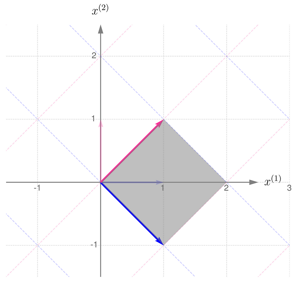
Here is the geometric interpretation of the transformation represented by the matrix A. The area shaded in gray is called the parallelogram.

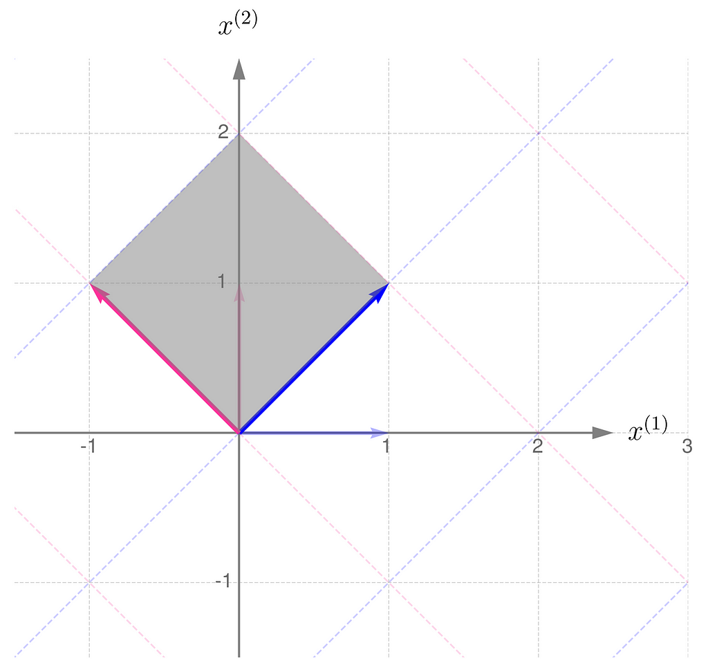
Compare this with the transformation obtained by applying the matrix Aᵀ:

Now, let us consider another transformation that applies entirely different scales to the unit vectors:

The parallelogram associated with the matrix B is much narrower now:

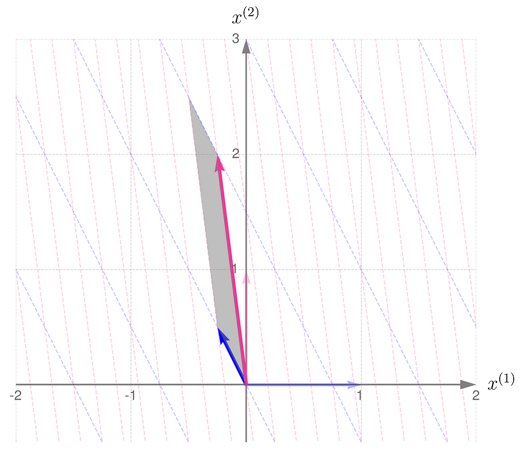
but it turns out that it is the same size as that for the matrix Bᵀ:

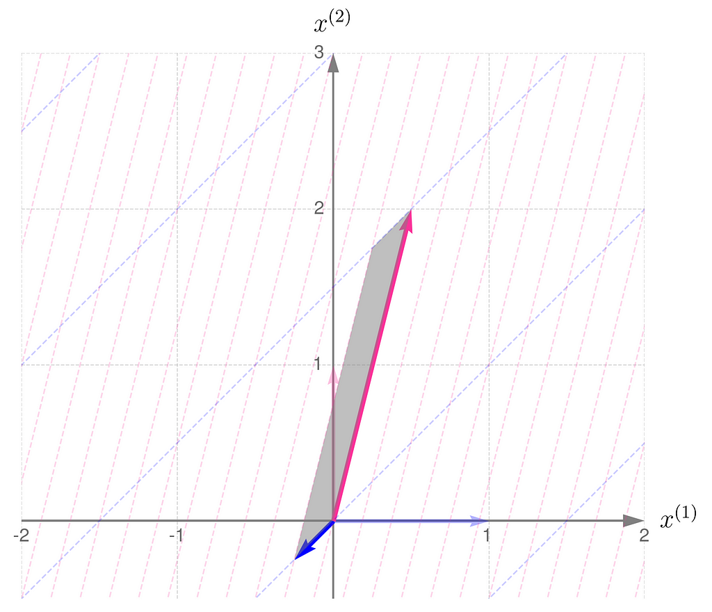
Let me put it this way: you have a set of numbers to assign to the components of your vectors. If you assign a larger number to one component, you’ll need to use smaller numbers for the others. In other words, the total length of the vectors that make up the parallelogram stays the same. I know this reasoning is a bit vague, so if you’re looking for more rigorous proofs, check the literature in the references section.

And here’s the kicker at the end of this section: the area of the parallelograms can be found by calculating the determinant of the matrix. What’s more, the determinant of the matrix and its transpose are identical.

More on the determinant in the upcoming sections.

5. Composition of transformations

You can apply a sequence of transformations — for example, start by applying A to the vector x, and then pass the result through B. This can be done by first multiplying the vector x by the matrix A, and then multiplying the result by the matrix B:

You can multiply the matrices B and A to obtain the matrix C for further use:

This is the effect of the transformation represented by the matrix C:

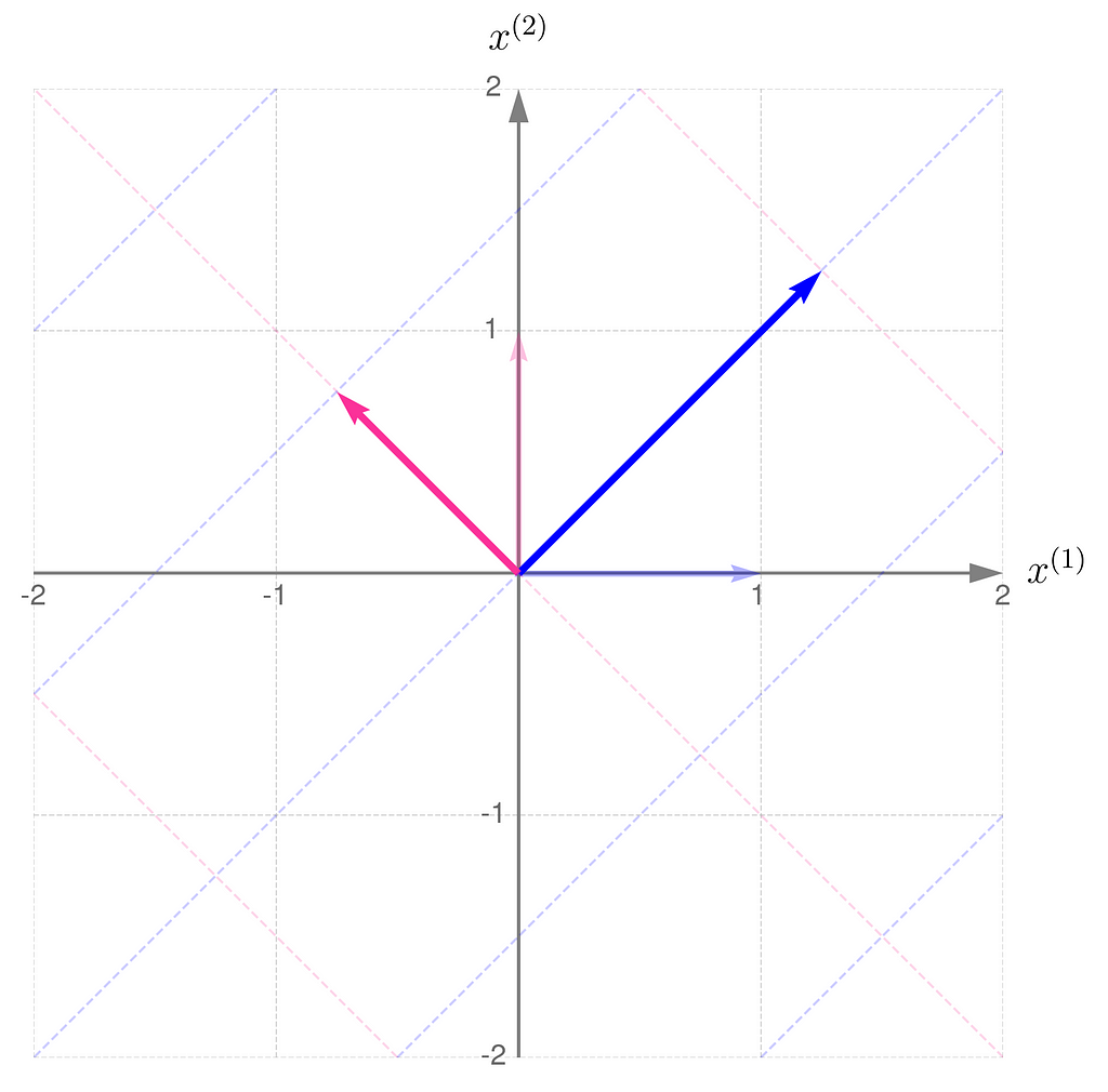
You can perform the transformations in reverse order: first apply B, then apply A:

Let D represent the sequence of multiplications performed in this order:

And this is how it affects the grid lines:

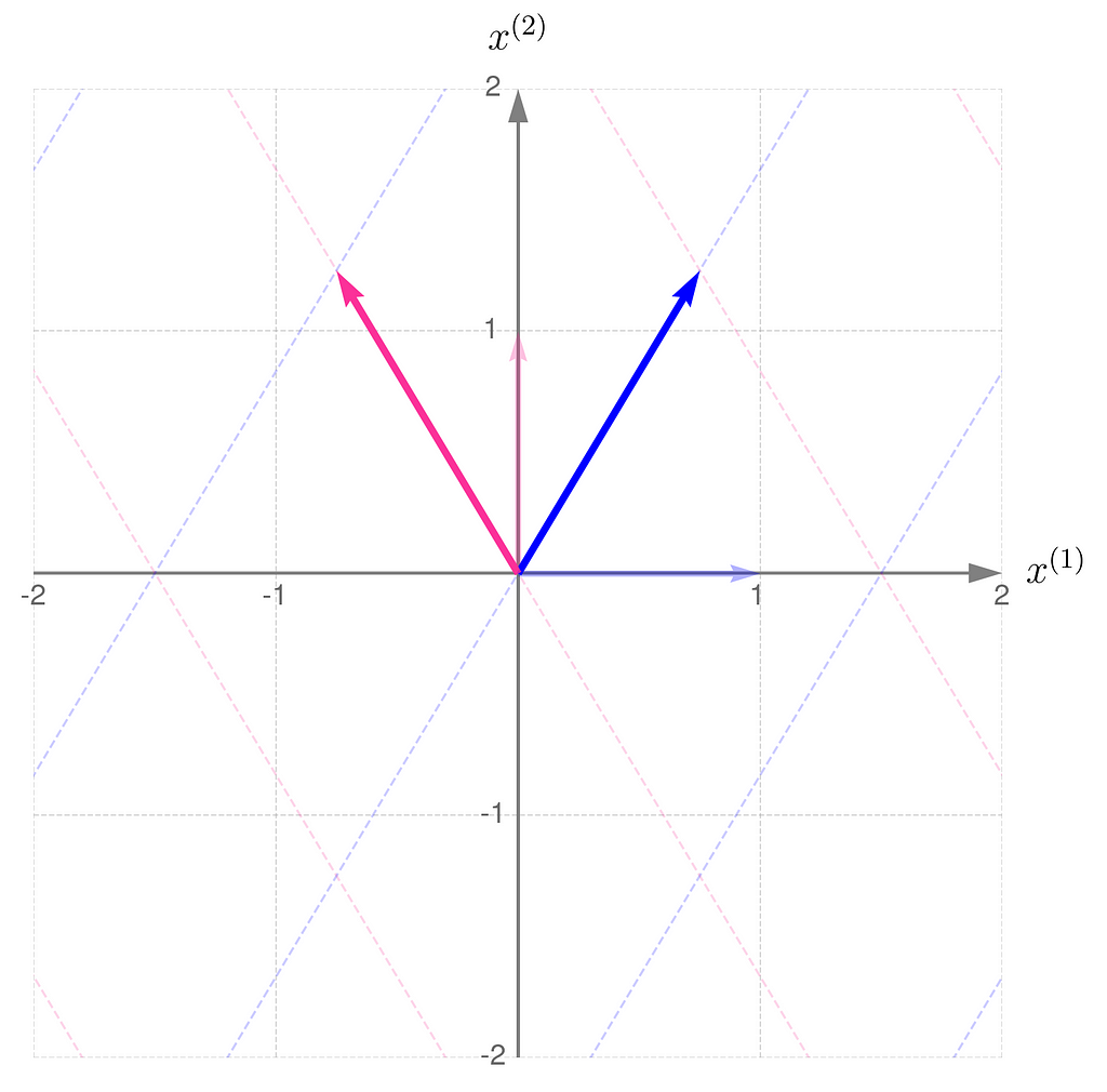
So, you can see for yourself that the order of matrix multiplication matters.

There’s a cool property with the transpose of a composite transformation. Check out what happens when we multiply A by B:

and then transpose the result, which means we’ll apply (AB)ᵀ:

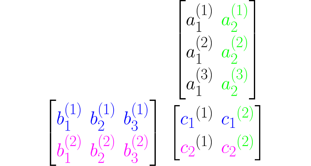
You can easily extend this observation to the following rule:

To finish off this section, consider the inverse problem: is it possible to recover matrices A and B given only C = AB?

This is matrix factorization, which, as you might expect, doesn’t have a unique solution. Matrix factorization is a powerful technique that can provide insight into transformations, as they may be expressed as a composition of simpler, elementary transformations. But that’s a topic for another time.

6. Inverse transformation

You can easily construct a matrix representing a do-nothing transformation that leaves the standard basis vectors unchanged:

It is commonly referred to as the identity matrix.

Take a matrix A and consider the transformation that undoes its effects. The matrix representing this transformation is A⁻¹. Specifically, when applied after or before A, it yields the identity matrix I:

There are many resources that explain how to calculate the inverse by hand. I recommend learning and was originally published in Towards Data Science on Medium, where people are continuing the conversation by highlighting and responding to this story.