Unlocking Hidden Potential: Exploring Second-Round Purchasers

Finding customer segments for optimal retargetting using LLM embeddings and ML model

Introduction

In this article, we are talking about a method of finding the customer segments within a binary classification dataset which have the maximum potential to tip over into the wanted class. This method can be employed for different use-cases such as selective targetting of customers in the second round of a promotional campaign, or finding nodes in a network, which are providing less-than-desirable experience, with the highest potential to move over into the desirable category.

Essentially, the method provides a way to prioritise a segment of the dataset which can provide the maximum bang for the buck.

The context

In this case, we are looking at a bank dataset. The bank is actively trying to sell loan products to the potential customers by runnign a campaign. This dataset is in public domain provided at Kaggle:

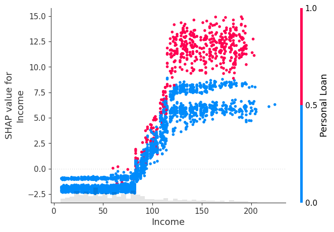
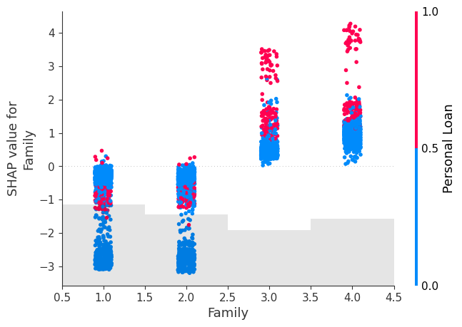
We will have a look at some of the important features as well to have an idea about the correlation with the dependent variable (‘Personal Loan’). The three features we have shortlisted for this purpose are ‘Income’, ‘Family’ (Family Size) and ‘Education’. As we will see later on, these are the features which we would want to keep our focus on to get the probability changed.

import shap

explainer = shap.Explainer(loaded_model, df_pred)
Shap_explainer = explainer(df_pred)
shap.plots.scatter(Shap_explainer[:, "Income"], color=Shap_explainer[:, "Personal Loan"])

shap.plots.scatter(Shap_explainer[:, "Family"], color=Shap_explainer[:,'Personal Loan'])

shap.plots.scatter(Shap_explainer[:, "Education"], color=Shap_explainer[:,'Personal Loan'])

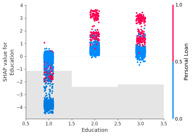
We see that for all 3 features, the purchase of Personal Loan increase as the feature value tends to increase, with Shap values of greater than 0 as the feature value increases indicating a positive impact of these features on the tendency to purchase.

We will now store the shap values for each of the customers in a dataframe so we can access the locally most important feature for later processing.

X_test = df_splitting(df_pred)[0] ## Keeping only the columns used for prediction
explainer = shap.Explainer(loaded_model.predict, X_test) 
Shap_explainer = explainer(X_test)
df_Shap_values = pd.DataFrame(Shap_explainer.values, columns=X_test.columns)
df_Shap_values.to_csv('Credit_Card_Fraud_Shap_Values.csv', index=False)

Step-3 : Creating Vector Embeddings:

As the next step, we move on to create the vector embeddings for our dataset using LLM model. The main purpose for this is to be able to do vector similarity search. We intend to find the customers in the dataset, who did not purchase the loan, who are closest to the customers in the dataset, who did purchase the loan. We would then pick the top closest customers and see how the probability changes for these once we change the values for the most important feature for these customers.

There are a number of steps involved in creating the vector embeddings using LLM and they are not described in detail here. For a good understanding of these processes, I would suggest to go through the below post by Damian Gill:

For us to get better vector embeddings, we would want to provide as much details about the data in words as possible. For the bank dataset, the details of each of the columns are provided in ‘Description’ sheet of the Excel file ‘Bank_Personal_Loan_Modelling.xlsx’. We use this description for the column names. Additionally, we convert the values with a little more description than just having numbers in there. For example, we replace column name ‘Family’ with ‘Family size of the customer’ and the values in this column from integers such as 2 to string such as ‘2 persons’. Here is a sample of the dataset after making these conversions:

def Get_Highest_SHAP_Values (row, no_of_values = 1):

    if row.sum() < 0:
        top_values = row.nsmallest(no_of_values)
    else:
        top_values = row.nlargest(no_of_values)
    return [f"{col}: {val}" for col, val in zip(top_values.index, top_values)]

def read_orig_data_categorized(categorized_filename, shap_filename = ''):

    df = pd.read_csv(categorized_filename)
    if shap_filename!= '':
        df_shap = pd.read_csv(shap_filename)
        df['Most Important Features'] = df_shap.apply(lambda row: Get_Highest_SHAP_Values(row, no_of_values = 1), axis=1)
    
    return df

def Column_name_changes (column_description, df):

    df_description = pd.read_excel(column_description, sheet_name='Description',skiprows=6, usecols=[1,2])
    df_description.replace('#','No of ', inplace=True, regex=True)
    df_description.replace('\(\$000\)','', inplace=True, regex=True)
    df_description.loc[df_description['Unnamed: 1']=='Education','Unnamed: 2'] = 'Education Level'
    mapping_dict = dict(zip(df_description['Unnamed: 1'], df_description['Unnamed: 2']))
    df = df.rename(columns=mapping_dict)

    return df


Original_Categorized_Dataset = r'Bank_Personal_Loan_Modelling_Semantic.csv' ## Dataset with more description of the values  sorted in the same way as df_pred and df_Shap_values
Shap_values_Dataset = r'Credit_Card_Fraud_Shap_Values.csv' ## Shap values dataset 
column_description = r'Bank_Personal_Loan_Modelling.xlsx' ## Original Bank Loan dataset with the Description Sheet

df_main = read_orig_data_categorized(Original_Categorized_Dataset, Shap_values_Dataset)
df_main = df_main.drop(columns=['ID','ZIP Code'])
df_main = Column_name_changes(column_description, df_main)
df_main.sample(5)

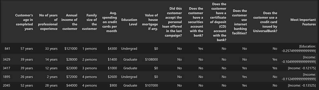
We will create two separate datasets — one for customers who purchased the loans and one for those who didn’t.

y_label_column = 'Did this customer accept the personal loan offered in the last campaign?'
df_main_true_cases = df_main[df_main[y_label_column]=="Yes"].reset_index(drop=True)
df_main_false_cases = df_main[df_main[y_label_column]=="No"].reset_index(drop=True)

We will create vector embeddings for both of these cases. Before we pass on the dataset to sentence transformer, here is what each row of the bank customer dataset would look like:

from sentence_transformers import SentenceTransformer

def df_to_text(row):

    text = ''
    for col in row.index:
        text += f"""{col}: {row[col]},"""
    return text

def generating_embeddings(df):

    sentences = df.apply(lambda row: df_to_text(row), axis=1).tolist()
    model = SentenceTransformer(r"sentence-transformers/paraphrase-MiniLM-L6-v2")
    output = model.encode(sentences=sentences,
            show_progress_bar=True,
            normalize_embeddings=True)
    df_embeddings = pd.DataFrame(output)

    return df_embeddings



df_embedding_all = generating_embeddings(df_main)
df_embedding_false_cases = generating_embeddings(df_main_false_cases)
df_embedding_true_cases = generating_embeddings(df_main_true_cases)

Step-4+5: Doing the Vector Search

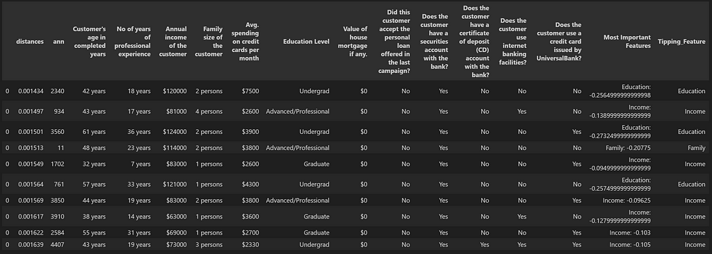
Next, we will be doing the Approximate Nearest Neighbor similarity search using Euclidean Distance L2 with Facebook AI Similarity Search (FAISS) and will create FAISS indexes for these vector datasets. The idea is to search for customers in the ‘Personal Loan = 0’ dataset which are most similar to the ones in the ‘Personal Loan = 1’ dataset. Basically we are looking for customers who did not purchase the loan but are most similar in nature to the ones who purchased the loan. In this case, we are doing the search for one ‘false’ customer for each ‘true’ customer by setting k=1 (one approximate nearest neighbor) and then sorting the results based on their distances.

Details about FAISS similarity search can be found here:

import faiss

def generating_index(df_embeddings):

    vector_dimension = df_embeddings.shape[1]
    index = faiss.IndexFlatL2(vector_dimension)
    faiss.normalize_L2(df_embeddings.values)
    index.add(df_embeddings.values)

    return index

def vector_search(index, df_search, df_original, k=1):

    sentences = df_search.apply(lambda row: df_to_text(row), axis=1).tolist()
    model = SentenceTransformer(r"sentence-transformers/paraphrase-MiniLM-L6-v2")
    output = model.encode(sentences=sentences,
            show_progress_bar=False,
            normalize_embeddings=True)
    search_vector = output
    faiss.normalize_L2(search_vector)
    distances, ann = index.search(search_vector, k=k)
    results = pd.DataFrame({'distances': distances[0], 'ann': ann[0]})
    df_results = pd.merge(results, df_original, left_on='ann', right_index= True)

    return df_results

def cluster_search(index, df_search, df_original, k=1):

    df_temp = pd.DataFrame()
    for i in range(0,len(df_search)):
        df_row_search = df_search.iloc[i:i+1].values
        df_temp = pd.concat([df_temp,vector_search_with_embeddings(df_row_search, df_original, index, k=k)])
    df_temp = df_temp.sort_values(by='distances')
    return df_temp

def vector_search_with_embeddings(search_vector, df_original, index, k=1):

    faiss.normalize_L2(search_vector)
    distances, ann = index.search(search_vector, k=k)
    results = pd.DataFrame({'distances': distances[0], 'ann': ann[0]})
    df_results = pd.merge(results, df_original, left_on='ann', right_index= True)

    return df_results

index_all = generating_index(df_embedding_all)
index_false_cases = generating_index(df_embedding_false_cases)
index_true_cases = generating_index(df_embedding_true_cases)

df_results = cluster_search(index_false_cases, df_embedding_true_cases, df_main_false_cases, k=1)
df_results['Most Important Features'] = [x[0] for x in df_results['Most Important Features'].values]
df_results ['Tipping_Feature'] = [x[0] for x in df_results['Most Important Features'].str.split(':')]
df_results = df_results.drop_duplicates(subset=['ann'])
df_results.head(10)

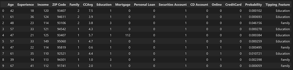
This gives us the list of customers most similar to the ones who purchased the loan and most likely to purchase in the second round, given the most important feature which was holding them back in the first round, gets slightly changed. This customer list can now be prioritized.

Step-6: A comparison with other method

At this point, we would like to assess if the above methodology is worth the time and if there can be another efficient way of extracting the same information? For example, we can think of getting the ‘False’ customers with the highest probabilities as the ones which have the highest potential for second round purchases. A comparison of such a list with the above list can be helpful to see if that can be a faster way of deriving conclusions.

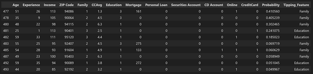
For this, we simply load up our dataset with the probabilities that we created earlier and pick the top 10 ‘False’ customers with the highest probabilities.

df_trial_customers = df_pred[df_pred['Personal Loan']==0].iloc[0:10]
df_trial_customers

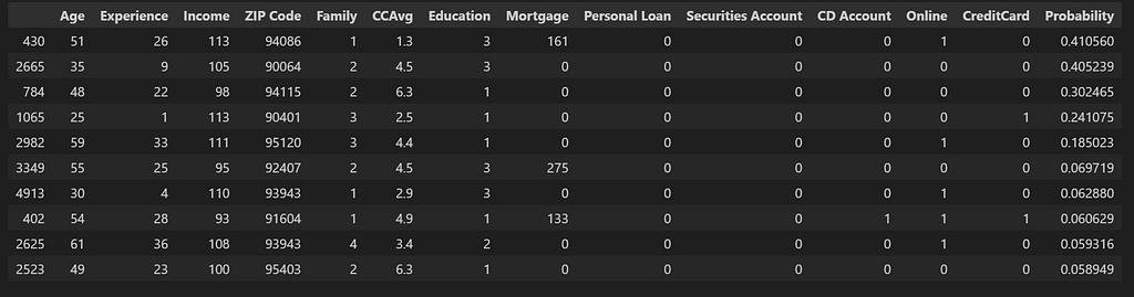
How effective this list is as compared to our first list and how to measure that? For this, we would like to think of the effectiveness of the list as the percentage of customers which we are able to tip over into the wanted category with minimal change in the most important feature by calculating new probability values after making slight change in the most important feature. For our analysis, we will only focus on the features Education and Family — the features which are likely to change over time. Even though Income can also be included in this category, for simplification purposes, we will not consider it for now. We will shortlist the top 10 candidates from both lists which have these as the Tipping_Feature.

This will give us the below 2 lists:

• List_A: This is the list we get using the similarity search method
• List_B: This is the list we get through sorting the False cases using their probabilities

features_list = ['Education', 'Family']
features_list = ('|').join(features_list)
df_list_A_Sim_Search = df_results[df_results['Tipping_Feature'].str.contains(features_list, case=False)].head(10)
df_list_A_Sim_Search

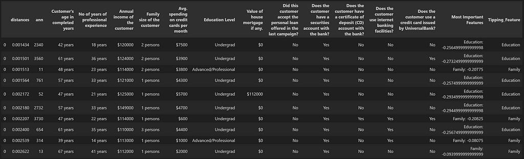
We will convert List_A into the original format which can be then used by the ML Model to calculate the probabilities. This would require a reference back to the original df_pred dataset and here is a function which can be used for that purpose.

def main_index_search(results_df, df_given_embeddings, df_original, search_index):
    
    df_temp = pd.DataFrame()
    for i in range(0,len(results_df)):
        index_number = results_df['ann'].iloc[i]
        df_row_search = df_given_embeddings.iloc[index_number:index_number+1].values
        df_temp = pd.concat([df_temp,vector_search_with_embeddings(df_row_search, df_original, search_index, k=1)])
    
    return df_temp

df_list_A_Sim_Search_pred = pd.concat([(main_index_search(df_list_A_Sim_Search, df_embedding_false_cases, df_pred, index_all).drop(columns=['distances','ann'])),\
                    df_list_A_Sim_Search ['Tipping_Feature']], axis=1).reset_index(drop=True)
df_list_A_Sim_Search_pred

Below is how we will get List_B by putting in the required filters on the original df_pred dataframe.

df_list_B_Probabilities = df_pred.copy().reset_index(drop=True)
df_list_B_Probabilities['Tipping_Feature'] = df_Shap_values.apply(lambda row: Get_Highest_SHAP_Values(row, no_of_values = 1), axis=1)
df_list_B_Probabilities['Tipping_Feature'] = [x[0] for x in df_list_B_Probabilities['Tipping_Feature'].values]
df_list_B_Probabilities ['Tipping_Feature'] = [x[0] for x in df_list_B_Probabilities['Tipping_Feature'].str.split(':')]
df_list_B_Probabilities = df_list_B_Probabilities[(df_list_B_Probabilities['Personal Loan']==0) & \
    (df_list_B_Probabilities['Tipping_Feature'].str.contains(features_list, case=False))].head(10)
df_list_B_Probabilities

For evaluation, I have created a function which does a grid search on the values of Family or Education depending upon the Tipping_Feature for that customer from minimum value (which would be the current value) to the maximum value (which is the maximum value seen in the entire dataset for that feature) till the probability increases beyond 0.5.

def finding_max(df):
    all_max_values = pd.DataFrame(df.max()).T
    
    return all_max_values

def finding_min(df):
    all_min_values = pd.DataFrame(df.min()).T
    
    return all_min_values

def grid_search(row, min_value, max_value, increment, tipping_feature):

    row[tipping_feature] = min_value
    row['New_Probability'] = [x[1] for x in loaded_model.predict_proba(row_splitting(row).convert_dtypes())][0]
    
    while (row['New_Probability']) < 0.5:

        if row[tipping_feature] == max_value:
            row['Tipping_Value'] = 'Max Value Reached'
            break

        else:
            row[tipping_feature] = row[tipping_feature] + increment
            row['Tipping_Value'] = row[tipping_feature]
            row['New_Probability'] = [x[1] for x in loaded_model.predict_proba(row_splitting(row).convert_dtypes())][0]
                
    return row

def row_splitting(row):
    prediction_columns = ['Age', 'Experience', 'Income', 'ZIP Code', 'Family', 'CCAvg',\
                          'Education', 'Mortgage', 'Personal Loan', 'Securities Account',\
                          'CD Account', 'Online', 'CreditCard']
    X_test = row.to_frame().transpose()
    X_test = X_test[prediction_columns].reset_index(drop=True)
    X_test = X_test.drop(columns=y_label_column)
    
    return X_test

def tipping_value(row, all_max_values, all_min_values):
    
    tipping_feature = row['Tipping_Feature']
    min_value = row[tipping_feature]
    max_value = all_max_values[tipping_feature].values[0]
    if tipping_feature == 'CCAvg':
        increment = 0.2
    else:
        increment = 1
    row = grid_search(row, min_value, max_value, increment, tipping_feature)
    row ['Value_Difference'] = row[tipping_feature] - min_value
    row ['Original_Value'] = min_value

    return row

min_values = finding_min(df_pred)
max_values = finding_max(df_pred)

df_new_prob = df_list_B_Probabilities.apply(lambda row: tipping_value(row, max_values, min_values), axis=1)
df_new_prob

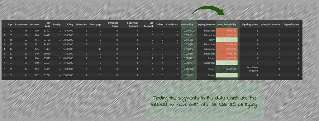
We see that with List B, the candidates which we got through the use of probabilities, there was one candidate which couldn’t move into the wanted category after changing the tipping_values. At the same time, there were 4 candidates (highlighted in red) which show very high probability of purchasing the loan after the tipping feature changes.

We run this again for the candidates in List A.

df_new_prob = df_list_A_Sim_Search_pred.apply(lambda row: tipping_value(row, max_values, min_values), axis=1)
df_new_prob

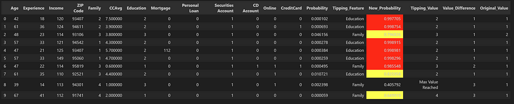
For List A, we see that while there is one candidate which couldn’t tip over into the wanted category, there are 6 candidates (highlighted in red) which show very high probability once the tipping feature value is changed. We can also see that these candidates originally had very low probabilities of purchasing the loan and without the use of similarity search, these potential candidates would have been missed out.

Conclusion

While there can be other methods to search for potential candidates, similarity search using LLM vector embeddings can highlight candidates which would most likely not get prioritized otherwise. The method can have various usage and in this case was combined with the probabilities calculated with the help of XGBoost model.

Unless stated otherwise, all images are by the author.

on Medium, where people are continuing the conversation by highlighting and responding to this story.