Mistral 7B Explained: Towards More Efficient Language Models

RMS Norm, RoPE, GQA, SWA, KV Cache, and more!

Part 5 in the “LLMs from Scratch” series — a complete guide to understanding and building Large Language Models. If you are interested in learning more about how these models work I encourage you to read:

• Part 5: Mistral 7B Explained: Towards More Efficient Language Models

Introduction

Mistral 7B was released in September 2023 and represents a significant milestone in the trend towards smaller, more efficient Large Language Models (LLMs). Over the last few years, the main improvement mechanism for LLM performance has been model size, that is, increasing the number of learnable parameters in the model. In recent times, this has given rise to models with hundreds of billions of parameters that incur higher training and serving costs as well as longer inference times. However, by leveraging careful architectural design and advancements in attention mechanisms, Mistral AI has pioneered the development of LLMs that achieve or even exceed the performance of much larger models using a fraction of the parameters. This article provides a comprehensive guide to the components inside Mistral 7B that enable these efficiency gains.

Note: In the next article, we will explore QLORA, a parameter-efficient fine-tuning technique, and show how to fine-tune both Mistral 7B and the enhanced NeMo 12B models for any downstream task.

Contents

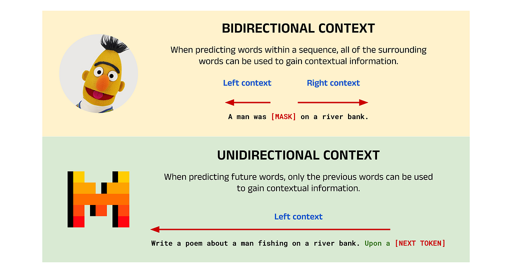
, we looked at Google’s BERT model, which is based on the encoder block of the original Transformer architecture. Encoder-only models are relatively uncommon outside of the BERT family of models, and most LLMs released after 2021 feature either the older encoder-decoder design of the original Transformer, or more commonly, the decoder-only architecture popularised by the original GPT. The encoder-only design allows BERT to make use of bidirectional context and excel in tasks such as classification. However, this design also restricts BERT’s ability in generative applications like chatbot tasks (which is likely the reason for the decline in encoder-only models).

In contrast, decoder-only models use unidirectional context to predict the next token in a sequence in a process known as Natural Language Generation (NLG). These models are used in chatbot applications such as virtual assistants, ChatGPT, etc., where users input prompts and the model generates appropriate responses one token at a time. As a model released after the BERT era, Mistral too uses a decoder-only architecture and is designed primarily for NLG tasks.

1.3 — Mistral 7B as an Efficient LLM

The Trend Towards Larger Models:

As previously mentioned, there has been a trend in the development of LLMs to improve performance by increasing model size. The general idea is that a larger model (a model with more parameters) can better capture relationships and subtleties in its training data, leading to better outputs during inference. This approach has proven incredibly effective, resulting in models that excel across all common performance benchmarks. Examples of these larger models include xAI’s Grok-1 (314 billion parameters), Google’s PaLM 2 (340 billion parameters), and OpenAI’s GPT-4, whose parameter count is not publicly disclosed but is believed to be in the trillions of parameters range.

Downsides of Larger Models:

While these larger models show high levels of performance, they also feature some notable downsides. Training these models is time-consuming and very expensive. The large number of parameters means that many weights and biases need to be updated in each optimisation step, requiring massive computational resources. This issue remains during inference, where prompting these models can result in slow response times without sufficiently power hardware. Other disadvantages include environmental and sustainability concerns due to the higher energy requirements, which increase their carbon footprint when compared to smaller models.

Mistral 7B as a Smaller, More Efficient Model:

Mistral 7B is well-known for its use of advancements in transformer architectures, which have allowed the model to maintain high performance while reducing the number of parameters. As a result, Mistral AI has been able to lead the development of efficient LLMs by taking the focus away from the current paradigm and instead promoting smaller models. This approach features several advantages, such as reducing training time and costs, as well as addressing the sustainability concerns described above. In the following sections, we will explore what these architectural changes are and how they allow for more performant models at smaller sizes.

1.4 — Overview of Base, Chat, and Instruct Models

Different Model Types:

If you have read around online about different LLMs, you may have come across the terms “base”, “chat”, and “instruct”. Base refers to the standard version of a model that can be fine-tuned on a downstream task, while chat and instruct refer to specific fine-tuned versions of base models that have been trained for chatbot and instruction tasks respectively. Chat models are fine-tuned on conversation data, and are designed for conversational chatbot applications such as virtual assistants and ChatGPT-style use-cases. Instruct models on the other hand are designed to receive instructions and respond to them. Though the two have slight differences in their fine-tuning (which are described below), it is important to recognise that the pre-training for both is identical. Hence, while each model is more performant in its respective area, it is possible to use either model for both tasks.

Chat vs. Instruct:

Chat models are designed for conversational interactions, aiming to simulate human-like conversations. For example, chat models often find use in virtual assistants in customer support settings, where the input format is more informal and flexible. In contrast, instruct models are designed to follow instructions and perform specific tasks based on those instructions. Examples here include tasks such as code generation and data summarisation. The input format for these types of models is more structured, requiring more formal prompts.

Model Types in Mistral 7B:

Mistral 7B is available in both base and instruct forms, though there is no specific version fine-tuned for chat available. However, the base version is very similar to the chat variants described above and can be interacted with in an unstructured, informal manner. To see a full list of Mistral AI models, you can visit the Mistral AI page on the Hugging Face model repository. [2]

1.5 — Performance on LLM Benchmarks

Mistral 7B can also be characterised by its strong performance compared to larger, contemporary models. In the initial promotional material, Mistral AI compared their new LLM to Meta’s Llama family of models: Llama and Llama 2 (Llama 3 had not been released at the time). The graphs of these performance comparisons are shown below and have been taken from the Mistral 7B paper [1].

Some of these benchmarks leverage zero-shot learning, few-shot learning, or a mixture of both. Zero-shot learning is the case where a model is asked to perform a task or answer questions based on data it has not explicitly encountered during pre-training. This requires the model to generalise from its existing knowledge to provide an answer. Few-shot learning, on the other hand, is the case where a model is provided with a few examples in the prompt to help it understand the format or type of answer expected.

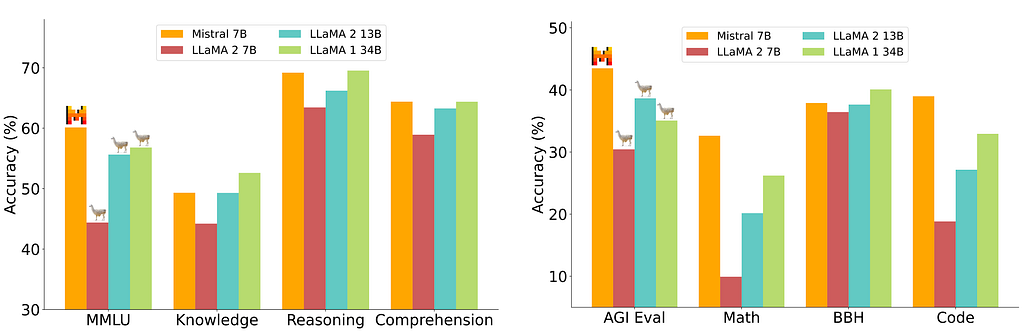
The overall trend shows that Mistral 7B outperforms Llama 2 13B across all metrics the models were evaluated on, often by a considerable margin. Perhaps more impressively, Mistral 7B also matches or exceeds the performance of Llama 1 34B in most benchmarks.

For the purpose of visualisation, the authors grouped some of the similar benchmarks together into categories, such as “Knowledge” and “Reasoning”. A breakdown of these categories is given below.

• MMLU: Massive Multitask Language Understanding (MMLU) is not a grouping but rather a single benchmark. This assessment is designed to measure how well a model has captured knowledge from its pre-training stage using both zero-shot and few-shot learning. The question set includes topics covering 57 subjects in science, technology, engineering, and mathematics (STEM), as well as the humanities, social sciences, law, ethics, and more. MMLU was introduced by Hendrycks et al. in 2021 and has been adopted by the NLP community as a de facto standard in evaluating LLM performance [3].
• Knowledge: The Knowledge category averages results from the NaturalQuestions and TriviaQA benchmarks using 5-shot learning. These datasets contain a series of questions to examine the general knowledge gained by a model from its training data.
• Reasoning: The Reasoning category averages results from the HellaSwag, Winogrande, PIQA, SIQA OpenbookQA, ARC-Easy, ARC-Challenge, and CommonsenseQA benchmarks using zero-shot learning. These datasets test a model’s ability to reason about the real world.
• Comprehension: The Comprehension category averages results from the BoolQ and QuAC benchmarks using zero-shot learning. These datasets focus on posing questions to a model based on passages of text in context, which evaluates a model’s ability to comprehend information in a dialogue.
• AGIEval: Like MMLU, AGIEval is a single benchmark and not a category of multiple benchmarks. AGIEval, short for Artificial General Intelligence Evaluation, is “specifically designed to assess foundation model[s] in the context of human-centric standardized exams, such as college entrance exams, law school admission tests, math competitions, and lawyer qualification tests”. The authors argue that previous benchmarks favour tasks suited to machines and artificial datasets, whereas AGIEval examines more human-level abilities. AGIEval was published in 2023 by Zhong et al. [4]
• Math: The Math category averages results from the GSM8K and MATH benchmarks, which use 8-shot and 4-shot learning respectively. These datasets contain mathematics questions with basic operations (addition, subtraction, multiplication, and division) and can take multiple steps to solve.
• BBH: Like MMLU and AGIEval, BIG-Bench Hard (shortened to BBH) is a single benchmark. BBH consists of 23 particularly challenging tasks from the larger BIG-Bench dataset, specifically focusing on evaluations where models did not outperform the average human rater. The benchmark was introduced in 2022 by Suzgun et al. [5]
• Code: The Code category averages results zero-shot Humaneval and 3-shot MBPP. These benchmarks assess the ability of a model to generate code from textual prompts.

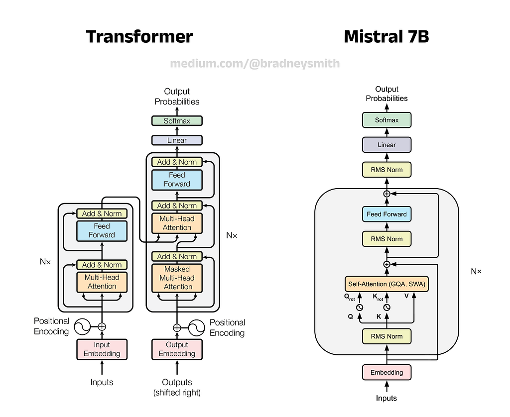
1.6— Mistral 7B Architecture Overview

LLM components have come a long way since the debut of the Transformer, and so modern LLMs often feature a number of improvements over the original design. Suggested improvements to attention mechanisms and positional encoders are being published reasonably frequently, with researchers racing to discover the next technique to push the art further.

In line with their mission, Mistral AI have utilised a number of these advancements to improve the efficiency of Mistral 7B, achieving a highly performant model with a fraction of the parameters. In the following sections we will explore these advancements, which include:

• RMS Normalization — replacing Layer Normalization
• Rotary Position Embedding (RoPE) — replacing Absolute Positional Encoding
• Grouped Query Attention (GQA) — replacing Multi-Head Attention
• Sliding Window Attention (SWA) — improving training and inference speed, particularly for long sequences
• Rolling Buffer KV Cache — improving training and inference speed, in conjunction with SWA
• SwiGLU Activation Function — replacing ReLU in the Feed Forward sub-layers

1.7 — BERT Parameter Comparison

Since the release of GPT and BERT in 2018, model sizes have continued to grow at a rapid pace, and it is not uncommon to see models with hundreds of billions of parameters. Compared to its contemporaries, Mistral 7B is considered a relatively small model. For perspective, BERT Large was considered incredibly large at the time of its release and contains only 340 million parameters, which shows how far the field has progressed in just a few years. For those following along with the series, you may recall a table in .

2. Embedding: Map each token to its corresponding learned embedding. These are vector representations of the tokens which encode their general meaning. For more about embeddings, see .

4. Normalization: Pass the contextual embeddings from the Attention block to the Normalization block. Here, the vectors of inputs are normalized to ensure a consistent mean and variance, mitigating the problem of covariate shift.

5. Feed Forward: Pass the output from the Normalization step to the Feed Forward sub-layer. This step updates the vector representation for each token in such a way that helps the model produce a nice poem later in the process. The specific steps for updating the vector representations are not hard-coded but rather learned by the model via backpropagation.

6. Normalization: Pass the outputs of the Feed Forward step to another Normalization block. Steps 3–6 repeat N times (where N is the number of encoder blocks) before the vector representations are sent to the decoder block.

2.2— Overview of Layer Normalization (LayerNorm)

The Transformer uses a type of normalization called LayerNorm, which was published in 2016 as an improvement to the older BatchNorm approach used by neural networks at the time [6]. The goal of LayerNorm is to prevent covariate shift by modifying the distribution of inputs to a layer so that they follow a Gaussian (Normal) distribution, hence the term “Normalization”.

Inputs to the Normalization Sub-Layer:

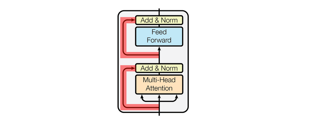
In the Transformer, the normalization process takes place after each Attention block and each Feed Forward block. Therefore, the inputs to the Normalization step will be different in each location:

• After Multi-Head Attention: Attention Input + Attention Output
• After Feed Forward: Feed Forward Input + Feed Forward Output

On first inspection, it may seem strange that the Normalization block is passed both the input to and output from the Attention/Feed Forward block. However, the inclusion of both of these components is critical to achieving strong model performance.

The Need for Residual Connections:

The architecture diagram below shows that inputs to the Attention and Feed Forward sub-layers are passed to the Normalization sub-layers via residual connections (highlighted in red). These inputs are added to the Attention and Feed Forward outputs respectively before normalization, hence the “Add” in the “Add & Norm” label. Residual connections help address an issue known as the vanishing gradient problem, a common challenge in training deep neural networks. During backpropagation, gradients (partial derivatives of the loss function with respect to each weight) determine the direction and magnitude of weight updates. However, these gradients can sometimes become extremely small as they propagate through many layers, leading to negligible changes in some weights. This can cause earlier layers in the network to learn very slowly as their gradients approach zero. Residual connections alleviate this problem by allowing gradients to flow more directly to earlier layers, bypassing some intermediate layers. This additional pathway helps maintain gradient strength, ensuring stable updates and preventing the model from “forgetting” what it has learned in earlier layers. In short, including a residual connection at each Normalization stage provides an additional path for backpropagated gradients and prevents the model from learning slowly in its earlier layers.

2.3 — Visualising LayerNorm

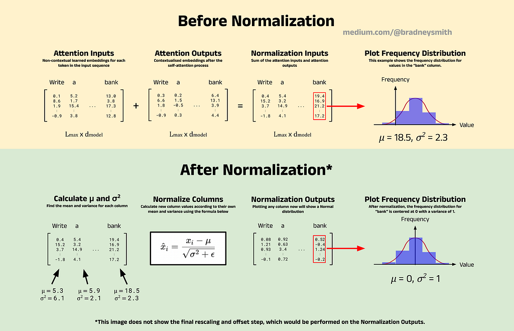
LayerNorm transforms the distribution of inputs to a network such that the values follow a Gaussian distribution. Consider the example shown in the image below, which focuses on Normalization directly after the Attention step. Here, the input to LayerNorm will be the sum of the Attention inputs and Attention outputs, the result of which is a matrix of contextual token embeddings for each token in the input sequence (in this case, “Write a poem about a man fishing on a river bank”). The dimensions of this matrix are L_max x d_model, where L_max is the input sequence length and d_model is the number of embedding dimensions. The columns of this matrix store the token embedding for each token of the input sequence. For example, the first column stores the contextual embedding for “write”, the second for “a”, and so on.

A frequency plot using a histogram can be drawn to approximate the distribution of values for each individual token embedding. The image below shows an example with the embedding for “bank.” Before normalization, the values in the embedding vector for “bank” have a mean of 18.5, whereas afterwards, the mean is reduced to 0. The normalization process is applied to each column of the matrix separately, with each normalized according to its own mean and variance.

2.4 — LayerNorm Formulae

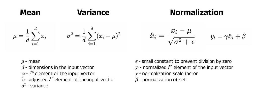
To normalize the token embeddings, we first calculate two key statistical values for each column: mean and variance. These values describe the centre and spread of the data, respectively. Once these have been established, each value in the input vector can be adjusted according to the normalization formula. Let’s briefly break down these formulae:

• Mean: The mean (average) describes the centre of a distribution and is calculated by summing all the values in a column and dividing by the number of values (dimensions) in the column.
• Variance: The variance describes the amount of spread (variation) within a distribution and is given by the average squared distance between each data point and the mean. A higher variance indicates that the data points are more spread out, while a lower variance indicates that the values cluster around the mean. The use of squared differences rather than absolute differences is partly due to historical reasons but also because it provides a differentiable measure of spread. This is a property that comes in very useful in advanced statistics, and so variance has become a standard measure in the field.
• Normalization: The normalization process involves two main formulae. The first (shown on the left of the two in the image below) transforms the column’s current distribution into a Normal distribution. This works by subtracting the mean from each value in the column so that the distribution is centred at 0, and then dividing by the square root of the variance (called the standard deviation). This division ensures the standard deviation of the resulting distribution is 1, which is a requirement for the Normal distribution. An additional term, ϵ, is included to prevent division by 0 when there is no spread in the data. The second formula applies learnable adjustments to these normalized values using two parameters: a scale factor, γ, and an offset, β. These parameters are learned by the model during training through backpropagation. The γ and β values are specific to each feature (row in the matrix), not to each embedding (column). Therefore, each dimension of an embedding will undergo a transformation using distinct γ and β values. This allows the model to learn flexible transformations within the embedding space, improving its ability to represent complex patterns in the data.

2.5— Introduction to RMS Normalization

Mistral 7B uses an improvement to LayerNorm called Root Mean Square Normalization, or RMS Norm, introduced by Zhang and Sennrich in 2019 [7]. The authors hypothesised that the effectiveness of LayerNorm was due to rescaling the values (dividing by the variance) and not so much recentering them (subtracting the mean).

Therefore, if the calculation of the mean could be omitted, the model would see a significant speed boost during the training phase. The issue here however, is that the calculation of the variance itself also requires the mean to be known. Hence, the authors set out to identify a new rescaling method that would become RMS Normalization.

2.6 — The RMS Statistic

The RMS statistic used to rescale the values has a simple formula, which is shown below. In essence, the value in each column of the input matrix (embedding) is divided by the square root of the average squared value in the column (hence “root mean square”). Similarly to LayerNorm, the results of the normalization are scaled by a learnable parameter, γ (note that β is not needed here since the authors argued that recentering is not necessary). Though a small change, replacing LayerNorm with RMS Norm results in a significant speed boost when training neural models, representing just one of many advancements in LLM architecture since the release of the Transformer.

3 — Rotary Position Embedding (RoPE)

3.1 — Overview of Positional Encoders

Unlike older architectures (such as Recurrent Neural Networks), Transformer-based models process all of their input tokens in parallel, not sequentially. While this parallel processing improves speed, it also results in a loss of positional information since the tokens are not processed in order. Therefore, some form of positional encoding is needed to inject this information back into the embedding vectors, and this can be achieved in various ways.

Absolute Positional Encoding:

The sinusoidal positional encoding technique introduced in the original Transformer uses sine and cosine functions to create a positional encoding vector for each token in the input sequence. These vectors are then added to the learned embeddings via vector addition. The positional encodings depend solely on the absolute position of the tokens in the sequence and do not change based on the input sequence itself. For example, the token at position 0 will always have the same positional encoding, regardless of the sequence. Hence, this method is called absolute positional encoding.

One limitation of this approach is that it only represents the absolute position of tokens, not their relative distances. For instance, the distance between the tokens in positions 3 and 5 of a sequence versus 103 and 105 is identical, but this information is not captured with absolute positional encoding. Intuitively, tokens that are closer together are likely to be more relevant than those that are further apart, and encoding this information about relative positioning could significantly improve model performance.

Relative Positional Encoding:

In April 2018, researchers at Google (including two authors of the original Transformer paper) published “Self-Attention with Relative Position Representations”, a paper that outlined a new paradigm for positional encoding [8]. The authors explored the use of relative positional encoding, which captures information about the relative distance between tokens as well as their absolute positions. For example, in the sentence “Write a poem about a man fishing on a river bank”, the words “poem” and “man” are three words apart, in the same way that “on” and “bank” are three words apart. This type of positional encoding has been used in prominent models such as Dai et al.’s Transformer-XL (2019) [9] and Google’s T5 (2020) [10].

Although relative positional encoding improves a model’s ability to capture the relationship between tokens, it significantly increases the training time. As models grow larger, adding components that increase training time becomes less practical. Additionally, challenges like integrating an KV cache (which we will cover later in this article) have caused many researchers to move away from this technique. We will not cover the details of the original relative positional encoding technique, but if you are interested, I highly encourage you to read through the paper.

Rotary Position Embeddings (RoPE):

Rotary embeddings were introduced by Su et al. in their 2020 paper “RoFormer: Enhanced Transformer with Rotary Position Embedding”, and offer a unique approach to encoding positional information [11]. Unlike sinusoidal encoding, which adds positional information directly to the token embeddings, rotary embeddings instead apply a rotation to the query and key vectors for each token. The rotation angle for each token is based on its absolute position in the sequence. For example, in the input “write a poem about a man fishing on a river bank”, the query and key vectors for poem (at position 2) are rotated by 2θ, while the query and key vectors for man (at position 5) are rotated by 5θ, and so on. Note that token position is zero-indexed, meaning we start counting at 0 instead of 1 (therefore write is said to be at position 0 and so its query and key vectors are not rotated). This approach captures not only the absolute position of the token but also the relative positions, since man and poem are 3θ apart, which represents a distance of 3 tokens.

Encoding positional information with angular displacement also offers a few nice properties that work well with existing transformer components. For example, the self-attention mechanism relies heavily on the dot-product operation, which already considers the angular distance between queries and keys in its formulae. Additionally, the angular distance between two tokens remains unchanged if more tokens are added before or after them. This allows for modifications to the input sequence without significantly altering the positional information, unlike the absolute positional encoding method.

3.2 — Implementing RoPE

The outline above gives a simplified overview of RoPE to illustrate its core concepts, but the technical implementation includes two important details:

1. Pair-wise feature rotation: The features of each query/key vector are rotated in pairs within the embedding space.

2. Multi-frequency positional encoding: Each feature pair in a query/key vector is rotated by a slightly different angle.

Let’s look at how RoPE integrates into transformer-based architectures, the mathematics behind its implementation, and understand what the two details above mean and why they are needed for RoPE to function effectively.

3.3 — Integrating RoPE into Transformers:

Transformers using RoPE process text with the following steps:

1. Tokenization and Embedding: As always, the process begins when a model receives an input sequence which is tokenized to produce a list of token IDs. These token IDs are then transformed into token embeddings, creating a matrix where each column corresponds to the embedding vector of a single token.

2. Normalization: In the original Transformer model, positional information is added directly to the raw token embeddings at this stage. However, in models using RoPE, the token embeddings are first normalized. This step stabilises training by preventing covariate shift, as discussed earlier (see the architecture diagram in Section 2.1).

3. Calculate Query, Key, and Value Matrices: The model then calculates the Query, Key, and Value matrices (Q, K, and V) needed for the attention mechanism. This is achieved by multiplying the normalized embeddings matrix by the corresponding weight matrices, W_Q, W_K, and W_V. Here, the columns of the resulting matrices represent the query, key, and value vectors for each token respectively. The Query and Key matrices are used to compute attention scores, which then weight the values in the Value matrix to produce context-aware outputs in the attention block (see , we covered the self-attention mechanism in detail and briefly introduced Multi-Head Attention (MHA), a specific implementation of self-attention from the original Transformer architecture. Since then, newer models have used improved attention mechanisms, optimising the efficiency of both training and inference. Mistral 7B uses Grouped Query Attention (GQA), which itself builds upon Multi-Query Attention (MQA). In this section, we will explore these techniques chronologically to understand how Mistral 7B performs self-attention.

4.1 — Overview of Multi-Head Attention (MHA)

Multi-Head Attention (MHA) was introduced in the 2017 paper “Attention is All You Need” [13] and extends standard self-attention by dividing the attention mechanism into multiple heads. In standard self-attention, the model learns a single set of weight matrices (W_Q, W_K, and W_V) that transform the token embedding matrix X into Query, Key, and Value matrices (Q, K, and V). These matrices are then used to compute attention scores and update X with contextual information.

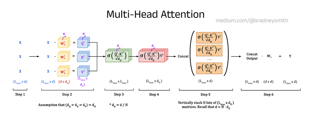
In contrast, MHA splits the attention mechanism into H independent heads, each learning its own smaller set of weight matrices. These weights are used to calculate a set of smaller, head-specific Query, Key, and Value matrices (denoted Q^h, K^h, and V^h). Each head processes the input sequence independently, generating distinct attention outputs. These outputs are then concatenated (stacked on top of each other) and passed through a final linear layer to produce the updated X matrix, shown as Y in the diagram below, with rich contextual information.

By introducing multiple heads, MHA increases the number of learnable parameters in the attention process, enabling the model to capture more complex relationships within the data. Each head learns its own weight matrices, allowing them to focus on different aspects of the input such as long-range dependencies (relationships between distant words), short-range dependencies (relationships between nearby words), grammatical syntax, etc. The overall effect produces a model with a more nuanced understanding of the input sequence.

4.2 — Multi-Head Attention Step-by-Step

Let’s walk through this process step by step, showing the equations used at each stage and their dimensions. A summary of these steps is given in a single diagram at the end.

1. Generate a Token Embedding Matrix, X:

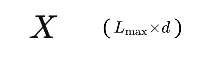
First, the input sequence is tokenized, the token IDs are mapped to their learned embeddings, and the positional information is added. This produces a matrix of size L_max x d, where L_max is the maximum length of the input sequence and d is the number of embedding dimensions for each token. This gives the token embedding matrix, X, which stores the token embedding vectors along its columns.

2. Calculate the Query, Key, and Value Matrices for each Head:

Next, the matrix X is passed to each head for processing. Every head has its own set of Query, Key, and Value weight matrices (denoted W_Q^h, W_K^h, and W_V^h), with dimensions d x d_H, where d_H is given by d/H. These weights matrices are pre-multiplied by X to give the Query, Key, and Value matrices (Q^h, K^h, and V^h) for the head, which have dimensions L_max x d_H.

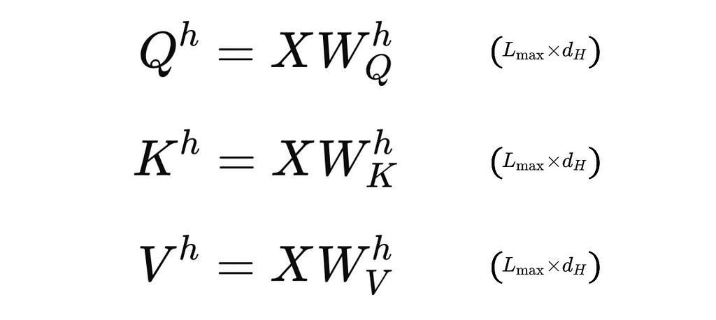
Note: In this explanation, we assume that W_Q^h, W_K^h, and W_V^h all have the same dimensions of d x d_H. This is not a strict requirement. In some implementations, the weight matrices for the Queries, Keys, and Values can have different numbers of columns, represented by d_Q, d_K, and d_V. In practice, however, it is most common to see d_Q = d_K = d_V = d_H, as we have here. It is useful to note that for this same reason, you will also see some people denote d_H simply as d_K (as we did in Part 3), since they are all equivalent.

3. Calculate the Attention Weights in Each Head:

For each head, the attention weights are calculated using the Query and Key matrices with the formula below, which produces a matrix with dimensions L_max x L_max. Using distinct weight matrices for each head allows them to capture different relationships in the sequence, such as syntactic or semantic patterns, improving the ability of the model to learn and generate text.

4. Calculate the Attention Outputs in Each Head:

In each head, the attention weights are used to pre-multiply the corresponding Value matrix, giving the matrix of attention outputs with dimensions L_max x d_H.

5. Concatenate the Attention Outputs:

The attention outputs from each head are then combined via concatenation. That is, a new matrix is constructed whose elements are simply the elements of attention outputs stacked on top of each other. The top of the matrix is populated by the outputs of the first head, then the second, and so on. Since this matrix is made up of H smaller matrices, each with dimensions L_max x d_H, the dimensions of the larger matrix are L_max x d (recall that d = H x d_h).

6. Apply Final Linear Transformation:

Finally, the concatenated matrix is processed through a linear layer, which can be expressed mathematically by the matrix multiplication below. The weights of this layer, W_O, are learned during training and transform the concatenated outputs into an output matrix Y. This output improves the representation of the input sequence given in X by improving the contextual information stored in the embeddings.

Summary of Multi-Head Attention:

The image below shows a summary of the MHA process:

4.3 — Multi-Query Attention (MQA)

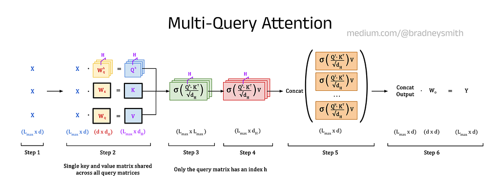
Multi-Head Attention has been shown to be very effective, producing state-of-the-art models since it was introduced in 2017. However, MHA suffers from one major drawback: the technique is incredibly memory-intensive. This is because large Key and Value matrices must be stored in memory for each attention head, causing a bottleneck that limits the overall model size that can be used with a given hardware setup. Multi-Query Attention (MQA) was proposed in 2019 to address this issue, debuting in the paper “Fast Transformer Decoding: One Write-Head is All You Need” by Noam Shazeer (one of the authors of the original Transformer) [14]. In MQA, the same Key and Value matrices are shared across all heads, and only the Query matrices are head-specific. This approach significantly reduces memory usage at the cost of a small reduction in performance. The diagram below shows the difference between the processes for MHA and MQA.

4.4 — Incremental Inference

The paper also describes an important optimisation technique called incremental inference, which is needed to improve the efficiency of LLMs as their sizes increase. In this approach, the model does not recalculate the Query, Key, and Value matrices for each timestep when predicting new tokens. Instead, the model makes use of cached values from the previous timestep. An outline of this process is given below:

1. Calculate Q_h, K, and V:

The model calculates a Query matrix for each attention head (Q_h) and shared Key (K) and Value (V) matrices for all heads based on the input sequence. The values in the K and V matrices are stored in a KV cache for use in subsequent attention calculations (we will discuss this more in Section 6). The values in the Q_h​ matrices are not cached because only the new token’s query vector will be needed in the next timestep (information about previous tokens is captured in K and V — see the database analogy in (2023), arXiv preprint arXiv:2310.06825.

[2] Hugging Face, (2020), arXiv preprint arXiv:2009.03300

[4] Zhong, W., et al., (2022) arXiv preprint arXiv:2210.09261.

[6] Ba, J., et al., (2019) preprint arXiv:1910.07467.

[8] Shaw, P., et al., (2019) arXiv:1901.02860.

[10] Raffel, C., et al., (2023) arXiv:2104.09864

[12] Hugging Face, (2017), Advances in Neural Information Processing Systems 30 (NIPS 2017)

[14] Shazeer, N., (2023) arXiv:2305.13245

[16] Raffel, C., et al., (2020) arXiv:2004.05150

[18] (2017) arXiv:1612.08083

[20] Chowdhery, A., et al, was originally published in Towards Data Science on Medium, where people are continuing the conversation by highlighting and responding to this story.