📚 The Perfect Way to Smooth Your Noisy Data

Insanely fast and reliable smoothing and interpolation with the Whittaker-Eilers method.

Real-world data is never clean. Whether you’re carrying out a survey, measuring rainfall or receiving GPS signals from space, noisy data is ever present. Dealing with such data is the main part of a data scientist’s job. It’s not all glamorous machine learning models and AI — it’s cleaning data in an attempt to extract as much meaningful information as possible. If you’re currently looking at a graph that has way too many squiggles to be useful. Well, I have the solution you’re looking for.

Whittaker-Eilers Smoothing

The Whittaker-Eilers smoother [1] was introduced to me when I was working in Earth Observation. Doing pixel-wise analysis on thousands of high-resolution satellite images requires insanely fast algorithms to sanitise the data. On any given day it might be cloudy, a few pixels may be obscured by smoke, or the sensor may have an artifact. The list can go on and on. What you’re left with is terabytes of rather noisy, gappy time-series data that needs to be smoothed and interpolated — and this is where the Whittaker smoother thrives.

Smoothing

Let’s start with a graph showing the global temperature anomaly between 1880 and 2022 [2]. In orange is the measured data and in green is the same data smoothed using the Whittaker-Eilers method.

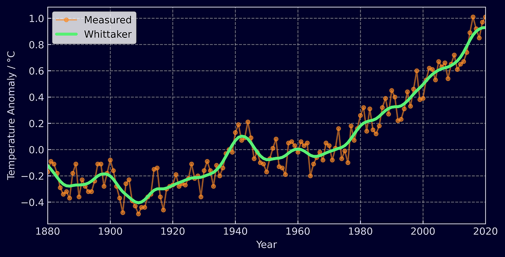
As you can see the raw time-series data is rather noisy. The conclusions we want to extract are not about year-to-year fluctuations but the general trend of the data over the past century. Smoothing the data offers a straight forward way to make the trend stand out and even better, it only takes 4 lines of code to run.

from whittaker_eilers import WhittakerSmoother

temp_anom = [-0.17, -0.09, -0.11, -0.18] # and so on...

whittaker_smoother = WhittakerSmoother(
    lmbda=20, order=2, data_length=len(temp_anom)
)

smoothed_temp_anom = whittaker_smoother.smooth(temp_anom)

If you’re not into Python, it’s only 4 lines of Rust code too.

use whittaker_eilers::WhittakerSmoother;

temp_anom = vec![-0.17, -0.09, -0.11, -0.18] // and so on...

let whittaker_smoother = 
            WhittakerSmoother::new(20, 2, temp_anom.len(), None, None)
            .unwrap();

let smoothed_data = whittaker_smoother.smooth(&temp_anom).unwrap();

Disclaimer, this is a package I’ve written — Python: pip install whittaker-eilers or Rust: cargo add whittaker-eilers

Interpolation

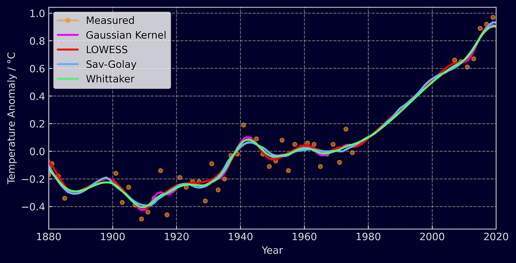
Now lets introduce some gaps into our data. Instead of having data that’s been uniformly collected each year, lets reduce it to every other year and add a couple of long gaps.

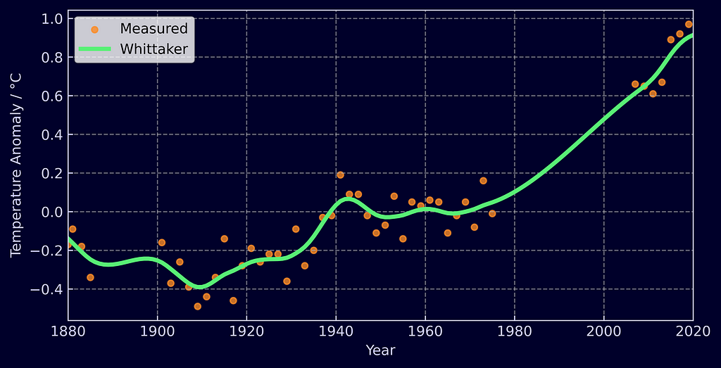
The Whittaker handles it effortlessly. All you need to do is assign a weight to each measurement. When interpolating, a measurement that exists is given a weight of 1 and a measurement you wish to obtain a value for is filled in with a dummy value, say -999, and assigned a weight of 0. The Whittaker handles the rest. It can also be used to accordingly weight measurements based on their uncertainty and can once again be deployed in a few lines of Python.

from whittaker_eilers import Whittaker

temp_anom = [-0.17, -0.09, -0.11, -0.18, -0.3] # and so on...
weights = [1.0, 0.0, 1.0, 0.0, 1.0]

whittaker_smoother = WhittakerSmoother(
    lmbda=150, order=2, data_length=len(temp_anom), weights=weights
)

smoothed_temp_anom = whittaker_smoother.smooth(temp_anom)

As well as gaps in the data, the Whittaker smoother can easily deal with unevenly spaced measurements. If you’re not bothered about interpolation and just want the smoothed values for the measurements you have, just provide an x_input containing when or where your measurements were taken. For example, [1880, 1885, 1886, 1900].

Configuration

With a single parameter, λ (lambda), you have continuous control over the smoothness of the data. The larger the lambda, the smoother the data.

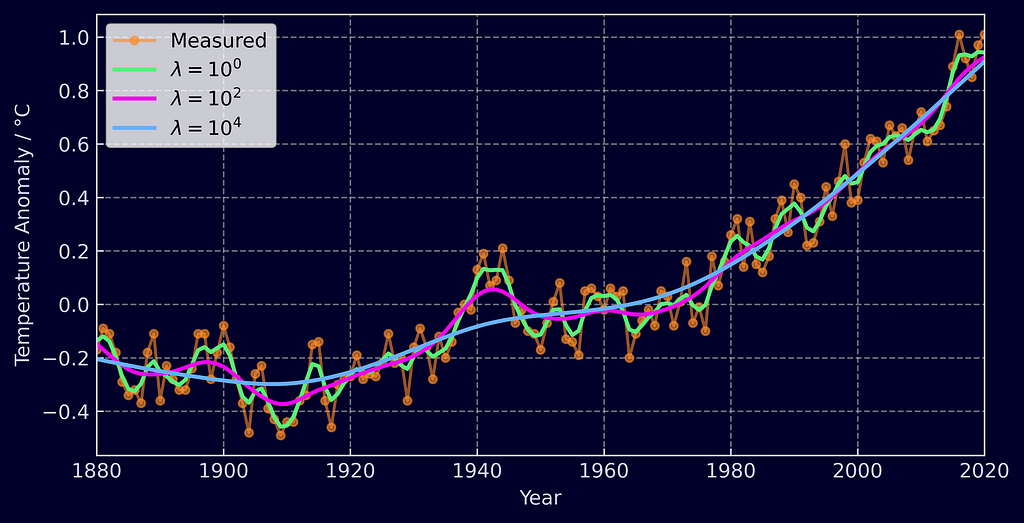
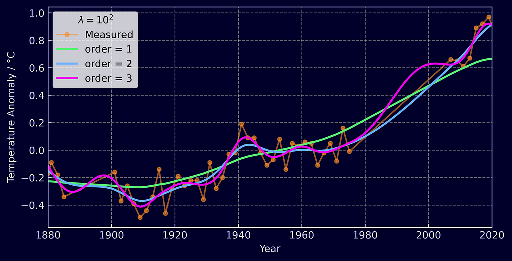
The order of the smoother, d, is also controllable. The higher the order, the more adjacent elements the Whittaker will take into account when calculating how smooth the time-series should be. The core take away from this is that interpolated data will be a polynomial of order 2d and extrapolated data will be of order d; though, we’ll dive into the mathematics of this a little later.

Comparison with other methods

To demonstrate how good the Whittaker-Eilers method is, let’s compare it against a few different techniques:

• Gaussian kernel smoothing (also known as an RBF kernel)
• Savitzky-Golay filter
• Local Regression (LOWESS)

The first is a kernel smoother, which essentially amounts to a fancy weighted average of neighbouring points. The second, the Savitzky-Golay filter is what Eilers’ original 2003 paper was positioning itself against and is very widely used. It smooths by carrying out a least squares fit of a polynomial to successive subsets of adjacent data. And finally, local regression which was the method of choice by NASA to smooth the temperature anomaly data seen above. This method performs iterative weighted linear fits on successive subsets of data, re-weighting the points based on the residuals as it goes.

I’ve opted not to include any methods aimed at real-time smoothing as they necessarily introduce a lag into your signal by only assessing past data. If you’re interested in such methods be sure to check out moving averages, exponential smoothers, and Kalman filters.

Smoothing

So let’s take a look at temperature anomaly time-series again, but this time smoothed with the additional methods.

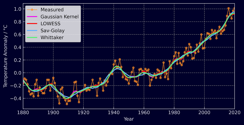
As you can see there’s not much variation — at least once you’ve got your parameters tuned. Let’s try an example that can tease out some differences as well as be benchmarked for performance. We’ll generate 4 basic sine waves between 0 and 2π and add some Gaussian noise to them. With each signal the sample size will increase, starting with 40 and finishing with 10,000. Already challenges are presented for the the Savitzky-Golay, Gaussian Kernel, and LOWESS methods. They expect a window length — some length of data that should be included in each successive subset to perform the fit/average on. If you’re increasing the number of measurements in the same space of time, you’ll need to make sure your window length varies with your overall data length to obtain optimal smoothing for each dataset. Below, each method roughly takes into account one tenth of the overall data for each window.

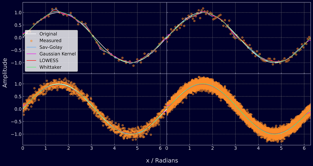
The Whittaker however does not need such dynamic parameter tuning. You can provide it with the measurement position x, set λ once, and you’ll be given smooth data every time. This knowledge of measurement position additionally enables it to handle unequally spaced data. LOWESS can also run on such data, but the other two methods require it to be equally spaced. Overall, I find the Whittaker the easiest to use.

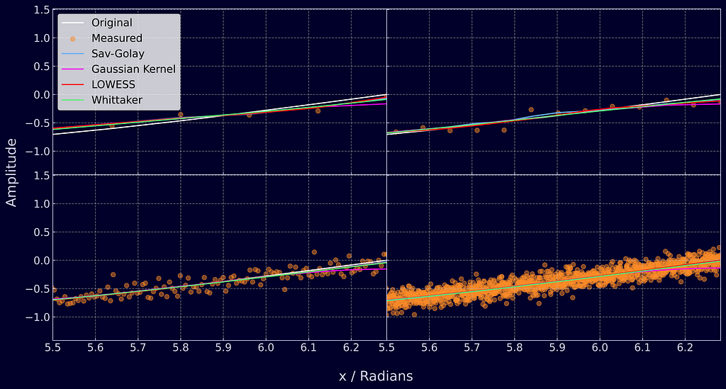
Another benefit of the Whittaker smoother is its adaptiveness to boundary conditions. At the edges of data, the Savitzky-Golay filter changes behavior as it can’t fit a polynomial past the end of the dataset without padding or mirroring it. Another option is to let it fit a polynomial to the final window and just use those results. The Gaussian kernel smoother struggles even more as no future measurements enter the average and it starts to exhibit a large bias from previous values, which can be clearly seen in the graph below.

Interpolation

A key feature of the Whittaker is its in-built ability to interpolate data. But how good is it compared to these other methods? The question isn’t clear-cut. Savitzky-Golay smoothing can interpolate, but only for gaps in data smaller than it’s window size and the same is true for LOWESS smoothing. Gaussian kernel smoothing doesn’t even have the ability to interpolate at all. The traditional solution to this problem is to apply linear interpolation to your data first and then smooth it. So we’ll apply this method to the other three techniques and compare the results against the Whittaker.

Each method will be compared against it’s own smoothed baseline taken from the graph at the start of this section (Figure 5). I removed every other point and introduced two large gaps, creating a dataset identical to the one seen in the interpolation example at the start of the article (Figure 2). For the baseline and interpolation runs the parameters were kept the same.

With linear interpolation filling in gaps, the methods perform well across the board. By calculating the Root Mean Squared Error (RSME) between the smoothed data without gaps and the smoothed data with gaps we get the following results.

• Linear Interpolation + Savitzky-Golay: 0.0245 °C
• Whittaker : 0.0271 °C
• Linear Interpolation + Gaussian kernel: 0.0275 °C
• Linear Interpolation + LOWESS: 0.0299 °C

The Savitzky-Golay method with linear interpolation gets the closest to the original smoothed data followed by the Whittaker, and there’s not much in it!

I’d just quickly like to mention that I've performed the interpolation benchmark this way, against their own smoothed baselines, to avoid tuning parameters. I could have used the sine wave with added noise, removed some data and tried to smooth it back to the original signal but this would have given me a headache trying to find the optimal parameters for each method.

Benchmarking

So lets revisit the sine wave data to generate some benchmarks of just how fast these methods are. I chose the most popular implementations in Python for each method. Savitzky-Golay and Gaussian kernel filters were implemented using SciPy, LOWESS was implemented from statsmodels, and the Whittaker from my Rust based Python package. The graph below shows how long each method took to smooth the sine wave with varying data lengths. The times reported are the sum of how long it took to smooth each dataset 50 times.

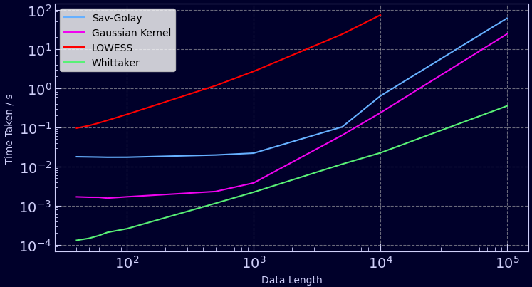
The quickest method by far is the Whittaker. It can smooth 50 time-series each 100,000 data points in length in under a second, 10 times faster than a Gaussian filter and 100 times faster than a Savitzky-Golay filter. The slowest was LOWESS even though it was configured not to iteratively re-weight each linear regression (an expensive operation). It’s worth noting that these methods can be sped up by adapting the window lengths, but then you’ll be sacrificing the smoothness of your data. This is a really great property of the Whittaker — its computation time increases linearly with data length (O(n)) and you never have to worry about window size. Furthermore, if you have gaps in your data you’ll be interpolating without any cost in speed whereas the other methods require some form of pre-processing!

The Mathematics

Now we’ve covered the top-line stuff, let’s dive into the maths behind the Whittaker-Eilers smoother and see why it’s such an elegant solution for noisy data [2] [3].

Imagine your noisy data y. There exists some series z which you believe to be of optimal smoothness for your y. The smoother z becomes, the larger the residuals between itself and the original data y. The Whittaker-Eilers method finds the optimal balance between these residuals and the smoothness of the data. The residuals are calculated as the standard sum of squared differences,

A metric for how smooth the data is can then be computed using the sum of squared differences between adjacent measurements,

S and R are the two properties we need to balance. But we also want to give the user control over where the right balance is, and we do this by introducing λ to scale the smoothness.

Now our goal becomes finding the series z that minimizes Q as this is where both the smoothness metric and residuals are at their minimum. Let’s expand Equation 3 and attempt to solve for z.

At this point it’s ideal to replace our summations with vectors,

We can then use a clever trick to represent Δz as a matrix and vector,

where m is the length of the data. If you matrix D against a vector, you’ll see it gives you the differences between adjacent elements — exactly what we want. We’re now left with a least squares problem. To find the minimum of Q we set its gradient to 0,

where I is the identity matrix (from factorizing z, a vector). We know I, D, λ and y, so we’re left with a simple linear equation,

which can be solved with any of your favourite matrix decompositions to achieve the smoothed data series z.

Interpolation

The above solution only accounts for evenly spaced data where all measurements are available. What about if you want interpolation? Well, you’ll need to apply weights to each of your measurements.

It’s as simple as revisiting Equation 1 and applying a weight to each residual and representing it as a diagonal matrix,

and then carrying out the same calculations as before,

Once again, this can be solved with a simple matrix decomposition, returning smoothed and interpolated data. All that needs to be done beforehand is to fill y with dummy values when an interpolated value is needed, such as -999, and set the weight of those measurements to 0 and watch the magic happen. Exactly how the data is interpolated depends upon the filter’s order.

Filter Order

The order of the Whittaker-Eilers smoother is something I touched upon in the configuration section. Now we have a mathematical framework for describing the smoother, it may make more sense. When creating R, our measure of smoothness, we first opted for “first-order” differences. We can quite easily take a second order difference where instead of penalizing our smoother based on adjacent data points, we can penalize it based on the change in first order differences, just like calculating a derivative.

This can then be expanded to third, forth, and fifth order differences and so on. It’s normally denoted as d and it’s not too tricky to implement as all that changes is the matrix D like so,

such that when it is multiplied with z, it expands into Equation 17. A simple function can be implemented to generate this matrix given a generic d.

Sparse Matrices

This can and has been implemented with sparse matrices as recommended by Eilers [1]. The matrices I and D are very sparsely populated and hugely benefit in terms of memory and computation if stored as sparse matrices. All of the maths presented above can be easily handled by sparse matrix packages, including Cholesky decompositions (and others). If not implemented with sparse matrices the algorithm can be incredibly slow for longer time-series, much slower than the other methods I compared it with.

Wrapping-up & Further Reading

This is an awesome algorithm and I can’t believe it isn’t utilized more. Weighted smoothing and interpolation wrapped up into fast, efficient matrix operations. What’s not to love?

I’ve included the Python scripts I used to carry out benchmarking and interpolation tests in the repo for the whittaker-eilers package. There’s also lots of examples showing you how to get started in Python or Rust as well as tests against Eilers’ original MATLAB algorithms [1]. But if you don’t care for that level of verbosity,

Python: pip install whittaker-eilers or Rust: cargo add whittaker-eilers

Even though this was a long post, I haven’t been able to cover everything here. Eilers’ 2003 paper also covers the mathematics behind smoothing unevenly spaced data and how cross-validation can be used to find an optimal λ. I’d recommend checking it out if you want to learn more about the maths behind the algorithm. I’d also suggest “Applied Optimum Signal Processing” by Sophocles J. Orfanidis as it offers an in-depth mathematical guide to all things signal processing. Thanks for reading! Be sure to check this post and others out on my personal site.

All images within this article have been produced by the author.

References

[1] Paul H. C. Eilers, A Perfect Smoother, Analytical Chemistry 2003 75 (14), 3631-3636, DOI: 10.1021/ac034173t

[2] NASA/GISS, Global Temperature, NASA’s Goddard Institute for Space Studies (GISS). URL: https://climate.nasa.gov/vital-signs/global-temperature/

[3] Sophocles J. Orfanidi, Applied Optimum Signal Processing, Rutgers University, URL: http://www.ece.rutgers.edu/~orfanidi/aosp

The Perfect Way to Smooth Your Noisy Data was originally published in Towards Data Science on Medium, where people are continuing the conversation by highlighting and responding to this story.